포물선

수학에서 포물선(parabola)은 대칭이며 거의 U자형인 평면 곡선이다.그것은 완전히 동일한 곡선을 정의한다는 것을 증명할 수 있는 표면적으로 다른 여러 수학적 설명에 들어맞는다.

포물선에 대한 한 가지 설명은 점(초점)과 선(직행렬)을 포함한다.초점은 다이렉트릭스에 있지 않다.포물선은 직행렬과 포커스에서 모두 등거리에 있는 평면에서 점의 궤적입니다.포물선에 대한 또 다른 설명은 오른쪽 원형 원뿔 표면과 원뿔 표면에 ^[a]접하는 다른 평면에 평행한 평면의 교차점에서 생성된 원뿔 단면입니다.

다이렉트릭스에 수직이고 포물선을 중앙을 통해 나누는 선(즉, 포물선을 나누는 선)을 "대칭의 축"이라고 합니다.포물선이 대칭축과 교차하는 점을 "버텍스"라고 하며 포물선이 가장 날카롭게 구부러진 지점입니다.대칭 축을 따라 측정된 정점과 초점 사이의 거리는 "초점 길이"입니다."직장직장"은 포물선의 현으로, 다이렉트릭스와 평행하며 포물선을 통과합니다.포물선은 위, 아래, 왼쪽, 오른쪽 또는 다른 임의의 방향으로 열릴 수 있습니다.모든 포물선은 다른 포물선에 정확히 맞도록 위치를 조정하고 크기를 조정할 수 있습니다. 즉, 모든 포물선은 기하학적으로 유사합니다.

포물선은 빛을 반사하는 물질로 만들어진 경우 포물선의 대칭축에 평행하게 이동하고 오목한 면을 타격하는 빛이 포물선의 어디에 반사가 발생하든 상관없이 포물선의 초점에 반사되는 특성이 있습니다.반대로 포커스의 점 소스로부터 발생하는 빛은 평행("시준") 빔에 반사되어 포물선이 대칭 축에 평행하게 유지됩니다.같은 효과가 소리와 다른 파동에서도 발생합니다.이러한 반사 특성은 포물선의 많은 실제 사용의 기초가 된다.

포물선은 포물선 안테나 또는 포물선 마이크에서 자동차 전조등 반사체 및 탄도 미사일 설계에 이르기까지 많은 중요한 응용 분야를 가지고 있다.그것은 물리학, 공학, 그리고 다른 많은 분야에서 자주 사용된다.

역사

원추형 단면에 대한 최초의 작품은 기원전 4세기에 메네크무스에 의해 알려졌다.그는 포물선을 이용하여 큐브를 두 배로 하는 문제를 해결할 방법을 발견했다.(단, 이 솔루션은 나침반과 직선 구조의 요건을 충족하지 않습니다.)포물선과 선분으로 둘러싸인 영역, 이른바 "포물선 세그먼트"는 기원전 3세기 아르키메데스에 의해 그의 포물선의 사각형에서 탈진 방법에 의해 계산되었다.파라볼라라는 이름은 원추형 단면의 많은 특성을 발견한 아폴로니우스 때문에 붙여졌다.이는 아폴로니우스가 ^[1]증명한 바와 같이 이 곡선과 관련이 있는 "영역의 적용" 개념을 가리키는 "적용"을 의미한다.포물선 및 기타 원뿔 섹션의 초점-직접성 특성은 파푸스 때문이다.

갈릴레오는 중력에 의한 균일한 가속의 결과로 발사체의 경로가 포물선을 따른다는 것을 보여주었다.

포물선 반사경이 이미지를 만들 수 있다는 생각은 반사 ^[2]망원경의 발명 이전에 이미 잘 알려져 있었다.디자인은 르네 데카르트와 마린 ^[3]메르센,^[4] 그리고 제임스 그레고리를 포함한 많은 수학자들에 의해 17세기 초중반에 제안되었다.아이작 뉴턴이 1668년에 최초의 반사 망원경을 만들었을 때, 그는 제작의 어려움 때문에 포물선 거울을 사용하는 것을 건너뛰었고, 구형 거울을 선택했다.포물선 거울은 대부분의 현대 반사 망원경, 위성 접시 및 레이더 ^[5]수신기에 사용됩니다.

점의 궤적으로서의 정의

포물선은 유클리드 평면에서 점 집합(점 위치)으로 기하학적으로 정의할 수 있습니다.

• 포물선은 점 세트입니다.$설정$된 점 P$({$$displaystyle$$$PF$})$에서 $F$({$displaystyle$F})까지의 ${\displaystyle \mathrm{거리}}$ P({displaystyle PF})가 직행렬인 $고정선$ L({$displaystyle$ L$\})$까지의 ${\displaystyle 거리}$ P${\displaystyle (\{}$displaystyle PF})와 같도록 합니다.

${\displaystyle\{P: PF = Pl \}$

$F$에서 $다이렉트릭스{\displaystyle }$ L$(Displaystyle$$$L$)$에 수직인 $중간점{\displaystyle }$ V$(Displaystyle$ V$)$를 정점이라고 하며, 선 $F{\displaystyle }$ $(Displaystyle FV)$는 포물선의 대칭축입니다.

데카르트 좌표계에서

Y축과 평행한 대칭축

만약 한 데카르트 좌표, 그러한 F)(0, f), f>;0,{\displaystyle F=(0,f),\ f>0,}과 준선은 방정식 y한 P점을 얻는다.)− f{\displaystyle y=-f},)소개하고 PF2)P나는 2{\displaystyle PF^{2}= Pl ^{2}}에서{P=(x, y)\displaystyle}(), y). 그 eq$uation{\displaystyle {}^{}}$ ${\displaystyle {x\mathrm{}}^{}}$2${\displaystyle }$+ (${\displaystyle y}$ -${\displaystyle {}^{}f}$ ) ${\displaystyle {2\mathrm{}}^{}}$ ${\displaystyle =}$ (${\displaystyle y}$ +${\displaystyle {}^{}f}$ ) ${\displaystyle {2\mathrm{}}^{}}${ { \ $displaystyle$ x$^{2$} + ( y - f )^{2} = ( $y$+ f$)^$2}$$$}.$ y {\ $displaystyle$ y$}$에 $대한{\displaystyle }$ 해결 결과

${\displaystyle y=snarfrac {1}{4f}}x^{2}.}$

이 포물선은 U자형(위쪽으로 열려 있음)입니다.

포커스를 통과하는 수평 코드(열림 부분의 그림 참조)를 라투스 직장이라고 하며, 그 절반은 반라투스 직장입니다.라투스 직장은 다이렉트릭스와 평행합니다.반라투스의 직장은$p{\displaystyle }$\$displaystyle$p로$$표기되어 있으며, 이 그림에서 알 수 있다.

$(\displaystyle p=2f).}$

라투스 직장은 타원과 쌍곡선이라는 다른 두 원뿔에 대해서도 비슷하게 정의됩니다.라투스 직장은 직교와 평행한 원뿔 단면의 초점을 통해 그려지고 곡선에 의해 양쪽 방향으로 종단되는 선입니다.$어느{\displaystyle }$ 경우든$$p\$displaystyle$p는$$ 정점에서의 원 반지름입니다.포물선의 경우 반직장인 $\displaystyle$p는$$다이렉트릭스로부터의 초점 거리입니다.$파라메타{\displaystyle }$p\$displaystyle$p를 사용하여 포물선의 방정식을 다음과 같이 다시 작성할 수 있습니다.

$(\displaystyle x^{2}=2py).}$

보다 일반적으로 $정점$이 V${\displaystyle =}$ ( ${\displaystyle {v\mathrm{}}_{}{1\mathrm{}}_{}}$ , ${\displaystyle {}_{}}$2 ) { $displaystyle$ V = ( $v$_ ${1$} , v$_$ {2}$$}인 경우, $초점{\displaystyle }$ ${\displaystyle {}_{}=}$ (${\displaystyle {}_{}{v\mathrm{}}_{}}$ ${\displaystyle {}_{}}$ ,${\displaystyle {}_{}{v\mathrm{}}_{}}$ ${\displaystyle 2}$+ f$$) { $displaystyle$ F $=$ ( v$_ {1$} , $v$_ ${2$} +$f$ )$$}$$the the $therixrixrixrixrixrixrixrixrix{\displaystyle }$ v $=$ $2$ - $f$、 { 2 - f$$。

${\displaystyle y=snarfrac {1}{4f}}(x-v_{1})^{2}+v_{2}=paramfrac {1}{4f}}x^{2}-{\frac {v_{1}{2f}x+{\frac {v_{1}^{2}}+v_{2}.}$

언급

1. f< { $display style$f < $0$}의 경우 포물선에는 아래쪽 개구부가 있습니다.
2. 축이 y축과 평행하다는 가정은 포물선을 2차 다항식의 그래프로 간주할 수 있으며, 반대로 2차 다항식의 그래프는 포물선이다(다음 절 참조).
3. x$(\displaystyle$ x$)$와$$y(\$displaystyle$ y$)$를 $교환$하면 y ${\displaystyle {2\mathrm{}}^{}}$ $=$ ${\displaystyle \mathrm{2p}}$x(\$displaystyle$ y$^{2$}= $2px$ $형식$의 방정식을 얻을 수 있습니다.이러한 포물선은 왼쪽(p \ $displaystyle$p <$0$) 또는 (> \ $displaystyle$ p $> 0$ )으로 열립니다.

일반 포지션

$초점$이 F${\displaystyle ={}_{}}$( ${\displaystyle {f\mathrm{}}_{}}$ ${\displaystyle {1\mathrm{}}_{}}$ ,$$f 2 ) { $displaystyle$ F = ($f$_ {$1}$ ,$f$ _$${2} $\}$ rixrixrixrixrix $directrix{\displaystyle }$ a${\displaystyle x}$ +${\displaystyle b}$ y + ${\displaystyle \mathrm{c}}$ $=$ 0 { $displaystyle$ ax $+ by$ + c$= 0$}이면 다음과 같은 식을 얻을 수 있습니다.

$(ax+by+c) 디스플레이 스타일^{2}}{a^{2}+b^{2}}=(x-f_{1})^{2}+(y-f_{2})^{2}}$

(이 방정식의 왼쪽은 헤세 정규 형태의 선을 사용하여 ${\displaystyle 거리}$ ${\displaystyle P}$ l$displaystyle$ Pl $}$을 계산합니다).

포물선의 일반적인 위치에 있는 파라볼라의 파라메트릭 방정식은 ② 단위 포물선의 아핀 이미지로 참조한다.

포물선의 암묵적 방정식은 2차 다항식으로 정의된다.

$({displaystyle ax^{2}+bxy+cy^{2}+cy+ey+f=0,}$

b ${\displaystyle {2\mathrm{}}^{}}$- ${\displaystyle 4}$ ${\displaystyle a}$ c ${\displaystyle =}$ $,$ {\$displaystyle$ b$^{2}-4ac=0,}$ $또는$ 이에 상당하는 ${\displaystyle {}^{}{2\mathrm{}}^{}}$ + ${\displaystyle b}$ ${\displaystyle x}$y + ${\displaystyle {}^{}}$ ${\displaystyle {y\mathrm{}}^{}}$2 {\$displaystyle$ ax$^{2}+bxy+cy^{2}}$가 선형 다항식의 제곱인 $경우{\displaystyle }$.

함수의 그래프로

이전 섹션은 원점을 정점으로 하고 y축을 대칭 축으로 하는 포물선을 함수의 그래프로 간주할 수 있음을 보여준다.

${\displaystyle f(x)=ax^{2}{\text{}a\neq 0.}}$

a> { $display$ $style$ a > $0$에서는 포물선이 위로 열리고, < $0$}에서는 포물선이 아래로 열립니다(그림 참조).위의 항에서 얻을 수 있는 것은 다음과 같습니다.

• 포커스는 ( ${\displaystyle 0\mathrm{}}$, ${\displaystyle 1\frac{\mathrm{}}{}}$ ${\displaystyle \frac{4}{}}$a$$) { $displaystyle \left$($0$, \ $frac${ 1$$} { 4 $a$} \ $right$ $。{\displaystyle }$
• 초점 $거리{\displaystyle \frac{\mathrm{}}{}}$ $4a({displaystyle {1$}{4a$\})$이며, 세미 라투스 ${\displaystyle 직장}$은 $p{\displaystyle }$ ${\displaystyle =}$ $2a$({$displaystyle$ p=$1blatus {$1}{2a$\}\}),$
• 정점은${\displaystyle }$( ${\displaystyle 0}$,${\displaystyle 0}$) {$displaystyle (0,0$
• directrix의 $공식$은 y $=$ - ${\displaystyle \frac{14\mathrm{}}{}}$ ${\displaystyle \frac{a}{}}${\$displaystyle$ y=-{\$frac {1}{4a$
• 점$({\displaystyle }$ x 0 , ${\displaystyle {}_{}}$ ${\displaystyle {}_{}^{}}$ 0${\displaystyle {}_{}}$2 )의$({displaystyle (x_{0,ax_{0}^2})$은 y ${\displaystyle =}$ ${\displaystyle 2}$ ${\displaystyle {a\mathrm{}}_{}}$ ${\displaystyle {}_{}}$- a ${\displaystyle {x\mathrm{}}_{}^{}}$ ${\displaystyle {\mathrm{}}_{}^{}}$ ${\displaystyle 2}$ $({$ y$=2ax_{0}x-ax_{0}^2$의 $방정식$을 가집니다.

a ${\displaystyle =}$({$displaystyle$ a$=1})$의 경우 포물선은 ${\displaystyle {y\mathrm{}}^{}}$ $=$ ${\displaystyle {}^{}}$({$displaystyle$ y$=x^{$2$\}\})$의 $단위{\displaystyle }$ 포물선입니다. 포물선의 초점은${\displaystyle }$(${\displaystyle 0\mathrm{},}$ 14$)$ {$displaystyle \left($$0{\displaystyle }$$,\tfrac$ {$1}{4}\right$ 반포물선 $p=$({$fract})$입니다.$({$ y$=-{\tfrac {1}{4$

도수 2의 일반적인 기능은

$f$(${\displaystyle x}$ ) ${\displaystyle =}$ ${\displaystyle {a\mathrm{}}^{}}$,${\displaystyle }$b , ${\displaystyle cr\mathbb{}}$R , ${\displaystyle \text{a}}$ ${\displaystyle 0}$0 {$display style$f ( x )$= a , b , c$\ $in$\$mathbb${ $R }$ , \$a$ \ $neq$ 0$$} .

제곱 수율 완성

${{displaystyle f(x)=a\left(x+{\frac {b}{2a}}\right)^{2}+{\frac {4ac-b^{2}}{4a}}}}$

포물선의 방정식인데

• $축{\displaystyle }$ x $=$ - ${\displaystyle \frac{b\mathrm{}}{}}$ 2$$ {\$display$ x=-{\$frac {b}{2a}}($Y 축에 위치),
• 초점 $거리{\displaystyle \frac{\mathrm{}}{}}$ $({$ $반직장{\displaystyle }$ p ${\displaystyle =}$ ${\displaystyle \frac{1\mathrm{}}{}}$ $({$ p$=squalfrac {1}{2a$
• $정점{\displaystyle }$ V ${\displaystyle =}$( - ${\displaystyle b\frac{}{}}$ ${\displaystyle \frac{2}{}}$ a${\displaystyle \frac{}{}}$, ${\displaystyle \frac{4a}{}}$ - ${\displaystyle \frac{{b\mathrm{}}^{}}{}}$ 2 ${\displaystyle \frac{{}^{}}{\mathrm{}}\frac{a}{}}$ )$${ $displaystyle$ V = \ $left$( - { \ $frac${ $b$} { $2a$} , { \ $frac${ $4ac$ - b^ {$2}}$ { 4a} } \ $right$$}$ ,
• $초점{\displaystyle }$ F ${\displaystyle =}$( - ${\displaystyle b\frac{}{}}$ ${\displaystyle \frac{2}{}}$a , ${\displaystyle \frac{4}{}}$a - ${\displaystyle \frac{{b\mathrm{}}^{}}{}}$2 + ${\displaystyle \frac{\mathrm{}}{}}$ 4${\displaystyle \frac{}{}\frac{a}{}}$) { $displaystyle$ F = \$left$ ( - { \ $frac${$b$} { $2a$} , { \ $frac${ $4ac$ - b^ {$2}$ +$1}$ { $4a}$ } \ $right$ ,
• $다이렉트릭스{\displaystyle }$ y ${\displaystyle =}$ ${\displaystyle 4\frac{\mathrm{}a}{}}$ - ${\displaystyle \frac{{b\mathrm{}}^{}}{}}$2 - ${\displaystyle \frac{1}{}}$ ${\displaystyle \frac{4}{}}$a {\$displaystyle$ y$=snapfrac {4ac-b^{2}-1}{4a$
• Y축과 교차하는 포물선의 점에는 좌표 $({\displaystyle 0}$ ${\displaystyle ,c}$) {$displaystyle (0,c$
• y축의 한 지점에서 접선의 $방정식$은 ${\displaystyle y}$ ${\displaystyle =b}$ x$$+ c {\$displaystyle y=bx+$c$\}$입니다.

유클리드 평면의 두 물체는 유사성, 즉 강체 운동(변환과 회전)의 임의 구성 및 균일한 축척에 의해 다른 물체와 변환될 수 있다면 유사하다.

$정점{\displaystyle }$ V ${\displaystyle =}$ ( ${\displaystyle {}_{}{}_{}}$1, ${\displaystyle {v\mathrm{}}_{}}$2)$${$displaystyle$ $V =$ ( $v_${1}, v_{2}}$${displaystyle V$$$=$ (${\displaystyle x}$ ,${\displaystyle y}$ ) ${\displaystyle \to }$ (${\displaystyle x}$ - v ${\displaystyle {1\mathrm{}}_{}}$, ${\displaystyle {y\mathrm{}}_{}}$ -$$2${\displaystyle {}_{}}$) { { $displaystyle ( x$ ,$y$ ) \ $to$( x - $v$_ 1$$} } { v _ y } { $v$} { v } { v } { v$$ } { v } { v } { displaysty } { v } { v }${\displaystyle }$} { $displaysty{\displaystyle \mathcal{}}$ } { displaysty } 원점을 중심으로 적절한 회전을 하면 포물선을 Y축을 대칭축으로 하는 포물선으로 변환할 수 있습니다.따라서 $포물선{\displaystyle \mathcal{}}$ P$(\$$style$$${$P$$})$는 y $=$ ${\displaystyle {a\mathrm{}}^{}}$ x 2, $0 0$의 $방정식$을 가진 포물선으로 강성운동으로 변환할 수 있습니다. 그런 포물선은 균일한 스케일링$({\displaystyle x}$,$y$ )$$ $,$ $)$로 변환할 수 $있습니다$.y ${\displaystyle =}$ ${\displaystyle {x\mathrm{}}^{}}$2 ({$style y=x^{$2$\}\})$인 ola. 따라서 모든 포물선을 단위 포물선에 유사성으로 ^[6]매핑할 수 있습니다.

유사한 삼각형을 사용하는 합성 접근법을 사용하여 이 결과를 ^[7]확립할 수도 있습니다.

그 결과, (필요하게 같은 유형의) 두 원뿔 단면이 같은 ^[6]편심인 경우에만 유사합니다.따라서 포물선(모두 편심 0)과 이 성질을 공유하는 것은 원뿐이며(모두 편심 1) 일반 타원 및 하이퍼볼라는 그렇지 않습니다.

$포물선{\displaystyle }$ y ${\displaystyle =}$ ${\displaystyle a}$ ${\displaystyle {x\mathrm{}}^{}}$2 {${\displaystyle }$$displaystyle$$$y =$ax^{2}$} and$$ 、 (${\displaystyle x}$, ${\displaystyle \frac{y}{}}$ )$$ ( $x$ , $y$) \ $to left$ ($x$ , { \ $tfrac${ $y$} { $a }$ }$$$\}{\displaystyle }$ 등 포물선 y = a x 2 를 유닛 포물선에 매핑하는 간단한 변환이 있습니다. 그러나 이 매핑은 모두 유사성을 나타내는 것은 아닙니다.s 단위 포물선의 아핀 영상).

특수 원뿔 섹션으로

x축을 대칭축으로 하고 원점(0, 0)에 있는 하나의 꼭지점 및 동일한 반직근 $(\displaystyle$ p$)$를 갖는 원뿔 단면 연필은 다음 방정식으로 나타낼 수 있다.

$\displaystyle y^{2}=2px+(e^{2}-1)x^{2},\display e\geq 0,}$

기괴한$모습$과 함께요$$

• e ${\displaystyle =}$ {$displaystyle$ e$=0}$의 경우 원뿔은 원(연필의 원추형 원)입니다.
• 0< < { $displaystyle$0 < $e }$ 타원에
• e ${\displaystyle =}$의 $경우{\displaystyle }$ {{$displaystyle$ e$=1}$ $방정식$이 ${\displaystyle {y\mathrm{}}^{}}$ 2 $=$ ${\displaystyle \mathrm{2p}}$x ,$${\$displaystyle$ y$^{2$}= $2px,}$인 포물선
• e> $(\displaystyle$ e$>1)$의 쌍곡선(그림 참조).

극좌표에서

$p{\displaystyle {}^{}}$ > 0이면 y ${\displaystyle {2\mathrm{}}^{}}$ $=$ ${\displaystyle 2}$ p ${\displaystyle x}${\$displaystyle$ y$^{2$}=$2px}($오른쪽 개구부)의 포물선이 극성을 나타낸다.

$\displaystyle r=2pfrac {cos \varphi }{\sin ^{2}\varphi },\display \varphi \in \left[-\tfrac {pi }{2},{\tfrac {2}},\setminus \{0\}$

( ${\displaystyle {r\mathrm{}}^{}}$ 2 ${\displaystyle {}^{}}$ ${\displaystyle {x\mathrm{}}^{}}$2 + ${\displaystyle {}^{}\text{2}}$ , ${\displaystyle x}$ $=$ ${\displaystyle r}$ cos${\$ {\ ${\displaystyle \mathrm{\phi display}}$ { $displaystyle$ r$^{2}$ = $x^{2$} + $y^{2}$ , \ x$= r$ \ cos \ $varphi }$ ) 。

정점은 $V{\displaystyle }$ ${\displaystyle =}$ (${\displaystyle }$0 ,${\displaystyle 0}$) { $displaystyle$ V = ($0$ , $0$)$$、 $F{\displaystyle }$ ${\displaystyle =}$ ( ${\displaystyle p\frac{}{}\frac{2}{}}$,${\displaystyle 0}$) { $displaystyle$ F = \ $left$( { \ $tfrac${ $p$} {2$}$ $, 0$ \ $right )$ $\}$ 。

원점을 포커스로 이동하면(${\displaystyle \mathrm{즉}}$, F${\displaystyle =}$( ${\displaystyle 0}$,$$0 ) {$displaystyle$ F$= (0,$0$)\}),$ 방정식을 얻을 수 있습니다.

${\displaystyle r=parfrac {p}{1-\cos \varphi }},\display \varphi \neq 2\pi k}$

비고 1: 이 극의 형태를 반전시키면 포물선이 심장의 역수임을 알 수 있습니다.

비고 2: 두 번째 폴라 형식은 $초점{\displaystyle }$ F ${\displaystyle =}$ ( ${\displaystyle 0}$,${\displaystyle 0}$) {$displaystyle$ F= ($0,0)}$의 원뿔 연필 케이스입니다(그림 참조).

${\displaystyle r}$ ${\displaystyle =}$ ${\displaystyle \frac{p\mathrm{}}{}}$1 - ${\displaystyle \frac{e}{}}$ cos ${\displaystyle \frac{}{}}$ φ$φ$ （ { $displaystyle$ r =$parfrac${$p$} { 1 -$$ \$cos$ \ $varphi }$ ）$$ ($$ { \ $displaystyle$ e$$}는$$ 편심입니다).

원뿔 단면 및 2차 형식

다이어그램, 설명 및 정의

이 다이어그램은 축이 AV인 원뿔을 나타냅니다.점 A는 그 정점입니다.분홍색인 원뿔의 경사단면은 원뿔의 측과 같은 각도θ만큼 축에서 경사져 있다.원뿔 단면으로서의 포물선의 정의에 따르면 이 분홍색 단면 EPD의 경계는 포물선이 된다.

원뿔의 축에 수직인 단면이 포물선의 정점 P를 통과한다.이 단면은 원형이지만 다이어그램에 표시된 것처럼 비스듬히 보면 타원형으로 나타납니다.중심은 V이고 PK는 직경입니다.반지름 r을 호출합니다.

원뿔의 또 다른 축에 수직인 원형의 단면은 앞에서 설명한 것보다 정점 A에서 멀리 떨어져 있다.포물선이 원과 교차하는 점을 연결하는 코드 DE가 있습니다.또 다른 현 BC는 DE의 수직 이등분선이며, 결과적으로 원의 지름이다.이 두 개의 화음과 포물선의 대칭축 PM은 모두 M 지점에서 교차합니다.

D와 E를 제외한 라벨이 붙은 모든 점은 동일평면이다.그것들은 전체 도형의 대칭면에 있다.여기에는 위에서 언급하지 않은 점 F가 포함됩니다.§ 포커스의 위치에서 다음과 같이 정의하고 논의합니다.

DM과 EM x의 길이, PM y의 길이를 호출합니다.

이차 방정식의 도출

BM과 CM의 길이는 다음과 같습니다.

${\displaystyle \stackrel{}{}}$${\displaystyle \stackrel{}{B}}$ M ${\displaystyle =}$ ${\displaystyle 2}$ ${\displaystyle y}$ sin ${\displaystyle =}$ 2 y sin ⁡$$（ $display$style ; $overline${ $mathrm {BM$} =$2$y \ $sin$\$theta$ （ BPM은 이등분이기 $때문$에 P M = ${\displaystyle \stackrel{}{A}}$ ${\displaystyle C\stackrel{}{}}$ ${\displaystyle ）}$ ${\displaystyle 、\mathrm{}}$ ${\displaystyle P}$ ${\displaystyle M}$ B ${\displaystyle =\mathrm{}A}$ ${\displaystyle \mathrm{style}}$ B$$= C ） ∠ C ∠ C 、 $Display$ ${\displaystyle B}$ ${\displaystyle \mathrm{（}}$ BPM ）

${\displaystyle \stackrel{}{\mathrm{C}}}$ M ${\displaystyle \stackrel{}{}}$ ${\displaystyle =}$ ${\displaystyle 2}$ ${\displaystyle r}$（ $display$;style $;style$ { $mathrm${$CM$} } =$2r$） (PMCK는 평행사변형).

코드 BC와 DE에서 교차하는 코드 정리를 사용하여, 우리는

${\displaystyle {\mathrm {BM}}\cdot {\mathrm {CM}=\cdot {\mathrm {DM}}\cdot {\mathrm {EM}}.$

대체:

$(\displaystyle 4ry\sin \theta =x^{2}).}$

재배치:

$({displaystyle y=snarfrac {x^{2}}){4r\sin \theta } } 。}$

주어진 원뿔과 포물선에 대해 r과 θ는 상수이지만, x와 y는 수평 단면 BECD가 만들어지는 임의의 높이에 의존하는 변수이다.이 마지막 방정식은 이러한 변수 간의 관계를 보여 줍니다.이들은 P를 원점으로 하는 분홍색 평면의 시스템에서 점 D와 E의 데카르트 좌표로 해석될 수 있다.x는 제곱이기 때문에 D와 E가 Y축의 반대편에 있다는 사실은 중요하지 않다.수평 단면이 원뿔의 꼭대기를 향해 또는 벗어나면 D와 E는 포물선을 따라 이동하며 항상 방정식에 표시된 x와 y의 관계를 유지합니다.따라서 포물선 곡선은 방정식이 만족되는 점의 궤적이므로 방정식에서 2차 함수의 데카르트 그래프가 됩니다.

초점 거리

그것은 이전 섹션에 포물선은 발신짔고 그것이 긍정적인 y방향으로 여는 꼭지점이 y=.mw-parser-output .sfrac{white-space:nowrap}.mw-parser-output.sfrac.tion,.mw-parser-output.sfrac .tion{은, 그 다음에 방정식은 증명되었다.디스플레이:inline-block, vertical-align:-0.5em, font-size:85%;text-align:센터}.mw-parser-output.sfrac.num,.mw-parser-output.sfrac .den{디스플레이:블록, line-height:1em, 마진:00.1em}.mw-parser-output.sfrac .den{border-top:1px 고체}.mw-parser-output .sr-only{.국경:0;클립:rect(0,0,0,0), 높이:1px, 마진:-1px, 오버 플로: 숨어 있었다. 패딩:0;위치:절대, 너비:f은 초점 거리 1px}x2/4f.[b]위의 마지막 방정식과 비교하면 원추형 포물선의 초점거리는 r sin θ이다.

포커스의 위치

위 다이어그램에서 V점은 포물선의 정점에서 원뿔의 축까지 수직의 발입니다.점 F는 점 V에서 포물선 ^[c]평면까지의 수직의 발입니다.대칭에 의해, F는 포물선의 대칭 축에 있다.각도 VPF는 θ를 보완하고 각도 PVF는 각도 VPF를 보완하므로 각도 PVF는 θ이다.PV의 길이가 r이므로 포물선의 정점에서 F의 거리는 r sin θ이다.위는 이 거리가 포물선의 초점 거리, 즉 정점에서 초점까지의 거리와 같다는 것을 보여준다.따라서 초점과 점 F는 같은 선을 따라 정점에서 동등하게 떨어져 있으며, 이는 같은 점임을 의미합니다.따라서 위에서 정의한 점 F는 포물선의 초점입니다.

이 논의는 포물선을 원뿔 단면으로 정의하는 것에서 시작되었지만, 이제 2차 함수의 그래프로 설명하게 되었다.이것은 이 두 가지 설명이 동일함을 나타냅니다.둘 다 정확히 같은 모양의 곡선을 정의합니다.

단델린 구를 사용한 대체 증거

다른 증거는 단델린 구를 사용하여 할 수 있다.계산 없이 작동하며 기본적인 기하학적 고려 사항만 사용합니다(아래 파생 참조).

수직으로부터의 기울기가 원뿔의 꼭대기와 점을 포함한 생성기(원뿔 표면의 선) $m{\displaystyle {}_{}}$0({디스플레이 스타일 ${0})$과 동일한 평면θ$(\$$displaystyle$ $\pi$ $\})$의 직립 원뿔의 교차점은 포물선(그림에서 빨간색)이다.

이 ${\displaystyle {generatrix\mathrm{}}_{}}$ m 0$({$$displaystyle$$m_$${$0$$$\})$은 $평면\theta$에 평행한 원뿔의 유일한 generatrix입니다$.$ $그렇지$ 않으면 교차 평면에 평행한 두 개의 generatrix가 있는 경우 교차 곡선은 쌍곡선이 됩니다(또는 두 개의 generatrix가 교차 평면에 있는 경우 퇴화 쌍곡선이 됩니다).교차 평면에 평행한 생성 행렬이 없는 경우 교차 곡선은 타원 또는 원(또는 점)이 됩니다.

$평면{\displaystyle }$ $「{displaystyle \sigma}」$를 원뿔의 수직축과 $라인{\displaystyle {}_{}}$ m ${$을 포함하는 평면이라고 합니다.수직으로부터의 평면 $(\displaystyle \pi)$는 라인 ${\displaystyle {m\mathrm{}}_{}}$ 0$(\$${0$$})$과 같습니다$.$, 측면(\$displaystyle$\$pi$$}$은 $평면$과 $수직{\displaystyle }$), ${\displaystyle m}$ 0 $}(\displaystyle$ $\sigma ）$$。$

포물선의 다이렉트트릭스 특성을 증명하기 위해(위의 "점 궤적으로서의 정의" 참조) Dandelin $spore{\displaystyle }$ d$\backslash$$displaystyle$ d를 사용합니다.Displaystyle d는 원 $\displaystyle$ c$}$ 및$$ 평면$$$\theta {\displaystyle }$\$displaystyle$$$F$\}$를 따라 원뿔과 접촉하는 구면이다.$e{\displaystyle }$ c$${\$displaystyle$ c$}$가 l$${\$displaystyle$ l$\}$ $라인$에서 $평면{\displaystyle }$ $"\displaystyle\pi"$와 교차합니다$$.시스템에는 $평면{\displaystyle }$ ${\$ { $displaystyle \pi$ $\}$ , Dandelin $sphere{\displaystyle }$d { $displaystyle$d$$ } 및 원뿔로 구성된 미러 대칭이 있습니다(대칭 평면은 $평면{\displaystyle }$ ${\$ { $displaystyle \sigma$}).$$

$\displaystyle$ c$\$$displaystyle\sigma$ 및$$ $c{\displaystyle }$\$displaystyle\sigma$를 포함하는$$ 평면은 $평면$과 수직이므로 $교차선{\displaystyle }$ l$\displaystyle$ l$\$$displaystyle$$\sigma$도 평면과$수직이어야$합니다$.$$$ 는 $평면{\displaystyle }$ $"\displaystyle\displaystyle$ $l{\displaystyle {\mu m\mathrm{}}_{}}$0 {\$displaystyle$ l$\perp m_{0$ 에 있습니다.

포물선의 초점은 F$(디스플레이$ 스타일 F$)$이고 포물선의 다이렉트릭스는$L(디스플레이$ 스타일 L$)$인 $것$으로 나타났습니다.

1. P$(\displaystyle$ P$)$를 교차 곡선의 임의의 점으로 $합니다{\displaystyle }$.
2. P$(\displaystyle$ P$)$를 $포함$하는 콘의 생성기는 $A{\displaystyle }$$(\displaystyle$ A$)$ $지점$에서 원$$c(\$displaystyle$ c$)$와 교차합니다$$.
3. $선분{\displaystyle \stackrel{}{}}$ ${\displaystyle \stackrel{}{P}}$ F ${\$ ( \ $display$style { $PF$} )${\displaystyle \stackrel{}{\mathrm{및<img\; alt="\{\backslash displaystyle\; \{\backslash overline\; \{PF\}\}\}"\; aria-hidden="true"\; class="mwe-math-fallback-image-inline"\; src="https://wikimedia.org/api/rest\_v1/media/math/render/svg/25ed728ba9ae9d5271c82809872bcbf3372c7a0f"\; style="vertical-align:\; -0.338ex;\; width:3.761ex;\; height:3.009ex;">}}}$ P A$display$ ( \ display$style$ { PA $}$ )는$$ 구$d{\displaystyle }$ ( \ $display style$d$$)에 접해 있기 때문에 길이가 같습니다.
4. $Generatrix{\displaystyle {}_{}}$ ${\displaystyle {m\mathrm{}}_{}}$ 0$({$이 $원{\displaystyle }$$$c$({$$displaystyle$D$\})$와 교차합니다$$. $선분{\displaystyle \stackrel{}{}}$ ${\displaystyle \stackrel{}{\mathrm{ZD}}}$ ${\({$와 ${\displaystyle \stackrel{}{\mathrm{ZA}}}${\({$displaystyle${$ZA$$\})$는$구$에 접하며, 따라서 길이가 같습니다.제1탄입니다.
5. $라인{\displaystyle }$q({$displaystyle$q}는$$${\displaystyle {m\mathrm{}}_{}}0$에 $평행$하고 포인트 P({displaystyle$m_$${0$$\})$를 ${\displaystyle \mathrm{통과}}$하는 라인입니다.${\displaystyle {m\mathrm{}}_{}}$ 0 $∥$ { $displaystyle$ m _ { 0 } \ $parallel$\ $pi$ $\}$ point 、$포인트{\displaystyle }$P$({displaystylel$ \ $pi$$\})$는 평면 $내$에 있으므로 $라인{\displaystyle }$ Q$({displaystyleline })$$가$$$ 있어야$$ 합니다.$0$${\displaystyle {}_{}}${ $displaystyle$ \ pi$$}.m 0$$ l { $displaystyle m$ _ {$0$ } \ $perp$l ${\displaystyle {m\mathrm{}}_{}}$ m 、 $q lstyle$ that \ that \ that ${\displaystyle \mathrm{that}}$ $that$$$。
6. $B를$$포인트$ P에서$$$L$까지의 수직의 발이라고 합니다.$즉{\displaystyle \stackrel{}{}}$, ${\$ { $displaystyle$ { $PB$$$}는 $Q$의 세그먼트이며, $따라서{\displaystyle \stackrel{}{}}$ ${\displaystyle \stackrel{}{\mathrm{PB}}over\stackrel{}{}\stackrel{}{Z}}$over { $displaystyle$ {$$PB$$}는 라인 Q의 세그먼트입니다$.$$ne {ZD$
7. ${\displaystyle \stackrel{}{\mathrm{가로채기}}}$ 정리와 ${\displaystyle \stackrel{}{Z}}$ D ${\displaystyle \stackrel{}{}}$ ${\displaystyle \stackrel{}{Z}}$ A $¯$ （ { $display$style$$${\displaystyle \stackrel{}{}}$ ${\displaystyle =}$ ${\displaystyle \stackrel{}{P}}$ B$$ ${\displaystyle \stackrel{}{}}$ $（$ \ $display$ style { $PA$ } =$PB$$）$ ¯ （ \ $display$ style ） = PB$$） ¯ （ \ display style ） ¯ ${\displaystyle =}$ $PB$（ \ $display$$$style${\displaystyle \stackrel{}{}}$） ¯¯¯¯ ¯ = ${\displaystyle PB\stackrel{}{}}$ ） ¯¯¯¯¯ ¯ ¯ ¯ ¯ ¯ ¯ ¯ ¯ ¯ ¯ ¯ ¯ ¯¯¯ ¯$play$style { $overline {PF$} =$overline {PB}$。이는 P$(\displaystyle$ P$)$에서 $포커스{\displaystyle }$ $(\displaystyle$ F$)$까지의 거리가 P$(\displaystyle$ P$)$에서 다이렉트릭스 $(\displaystyle$ l$)$까지의 거리와 같다는 것을 의미합니다.

반사 특성은 포물선이 빛을 반사할 수 있는 경우, 포물선에 들어간 빛이 대칭축과 평행하게 이동하면서 초점을 향해 반사된다는 것을 나타냅니다.이것은 빛이 광선을 통과한다는 가정에 기초한 기하학적 광학에서 도출됩니다.

포물선 y = x를² 고려합니다. 모든 포물선이 유사하므로 이 간단한 사례는 다른 모든 경우를 나타냅니다.

와

점 E는 포물선상의 임의의 점입니다.초점은 F, 정점은 A(원점), 선 FA는 대칭의 축입니다.선 EC는 대칭 축과 평행하며 D에서 x 축과 교차합니다.점 B는 회선 세그먼트 FC의 중간점입니다.

제제

정점 A는 초점 F 및 직행렬에서 등거리에 있습니다.C는 직행렬 상에 있으므로 F와 C의 y 좌표는 절대값이 같고 부호는 반대이다.B는 FC의 중간 지점입니다.x좌표는 D의 절반, 즉 x/2입니다.선 BE의 기울기는 ED 및 BD 길이의 몫이며, 이는 x/x/2 = 2x입니다². 그러나 2x는 E에서 포물선의 기울기(제1도함수)이기도 합니다.따라서 선 BE는 E에서 포물선에 대한 접선입니다.

E는 포물선에 있고 F는 포커스에 있으며 C는 직행렬에 있으므로 EF와 EC의 거리는 같다.따라서 B는 FC의 중간점이므로 삼각형 △ FEB와 △ CEB는 일치하며, 이는 α로 표시된 각도가 일치함을 의미한다(E 위의 각도는 수직으로 반대되는 각도 θBEC).즉, 포물선에 들어가 대칭 축에 평행하게 이동하는 E에 도달하는 광선이 라인 BE에 반사되어 다이어그램에서 빨간색으로 표시된 것처럼 라인 EF를 따라 이동합니다(라인은 어떻게든 빛을 반사할 수 있다고 가정).BE는 E에서 포물선에 대한 접선이기 때문에, 같은 반사가 E에서 포물선의 극소 호에서 이루어집니다.따라서 포물선에 들어가 포물선의 대칭축과 평행으로 이동하는 E에 도달하는 빛은 포물선에 의해 포물선의 초점을 향해 반사됩니다.

반사광에 대한 이 결론은 다이어그램의 왼쪽에서 볼 수 있듯이 포물선의 모든 점에 적용됩니다.이것은 반사 특성입니다.

기타 결과

위의 주장에서 간단히 추론할 수 있는 다른 이론들이 있다.

접선 이등분 특성

위의 증명과 부수되는 그림은 탄젠트 BE가 각도θFEC를 이등분하고 있음을 보여준다.즉, 임의의 점에서의 포물선에 대한 접선은 점을 포커스에 연결하는 선 사이의 각도를 직각으로 이등분합니다.

접선과 포커스에서 수직인 교차점

삼각형 △FBE와 △CBE는 합동이므로 FB는 탄젠트 BE에 수직입니다.B는 정점의 포물선에 대한 접선인 x축에 있으므로 포물선에 대한 접선과 포물선에 대한 포커스에서 수직 사이의 교차점은 정점의 포물선에 접하는 선에 있습니다.애니메이션^[8] 다이어그램 및 페달 곡선을 참조하십시오.

볼록한 면에 부딪히는 빛의 반사

만약 빛이 CE선을 따라 이동한다면, 그것은 대칭축에 평행하게 움직이며 포물선의 볼록한 면을 E로 친다.위의 도표에서 이 빛이 세그먼트 FE의 확장을 따라 포커스에서 직접 반사되는 것이 명확합니다.

대체 증명

반사 및 접선 이등분 특성에 대한 위의 증명은 미적분을 사용합니다.여기에 기하학적 증거가 제시되어 있다.

이 그림에서 F는 포물선의 초점이고 T와 U는 포물선의 직행렬 위에 있다.P는 포물선상의 임의의 점입니다.PT는 다이렉트릭스에 수직이며, MP 이등분선각θFPT이다.Q는 포물선의 또 다른 점이며, QU는 직각 행렬에 수직입니다.FP = PT 및 FQ = QU임을 알 수 있습니다. 분명히 QT > QU이므로 QT > FQ입니다.이등분선 MP의 모든 점은 F와 T에서 등거리이지만 Q는 T보다 F에 가깝다.즉, Q는 MP의 왼쪽에 있습니다.즉, 포커스와 같은 쪽에 있습니다.Q가 포물선의 다른 곳(P점 제외)에 있는 경우에도 마찬가지입니다. 따라서 P점을 제외한 전체 포물선은 MP의 초점 쪽에 있습니다. 따라서 MP는 P에서 포물선에 접하는 접선입니다.각도θFPT를 이등분하기 때문에 이는 접선 이등분 특성을 증명한다.

The logic of the last paragraph can be applied to modify the above proof of the reflective property. It effectively proves the line BE to be the tangent to the parabola at E if the angles α are equal. The reflective property follows as shown previously.

Pin and string construction

The definition of a parabola by its focus and directrix can be used for drawing it with help of pins and strings:^[9]

1. Choose the focus ${\displaystyle F}$ and the directrix ${\displaystyle l}$ of the parabola.
2. Take a triangle of a set square and prepare a string with length ${\displaystyle AB }$ (see diagram).
3. Pin one end of the string at point ${\displaystyle A}$ of the triangle and the other one to the focus ${\displaystyle F}$.
4. Position the triangle such that the second edge of the right angle is free to slide along the directrix.
5. Take a pen and hold the string tight to the triangle.
6. While moving the triangle along the directrix, the pen draws an arc of a parabola, because of ${\displaystyle PF = PB }$ (see definition of a parabola).

Properties related to Pascal's theorem

A parabola can be considered as the affine part of a non-degenerated projective conic with a point ${\displaystyle Y_{\infty }}$ on the line of infinity ${\displaystyle g_{\infty }}$, which is the tangent at ${\displaystyle Y_{\infty }}$. The 5-, 4- and 3- point degenerations of Pascal's theorem are properties of a conic dealing with at least one tangent. If one considers this tangent as the line at infinity and its point of contact as the point at infinity of the y axis, one obtains three statements for a parabola.

The following properties of a parabola deal only with terms connect, intersect, parallel, which are invariants of similarities. So, it is sufficient to prove any property for the unit parabola with equation ${\displaystyle y=x^{2}}$.

4-points property

Any parabola can be described in a suitable coordinate system by an equation ${\displaystyle y=ax^{2}}$.

• Let ${\displaystyle P_{1}=(x_{1},y_{1}),\ P_{2}=(x_{2},y_{2}),\ P_{3}=(x_{3},y_{3}),\ P_{4}=(x_{4},y_{4})}$ be four points of the parabola ${\displaystyle y=ax^{2}}$, and ${\displaystyle Q_{2}}$ the intersection of the secant line ${\displaystyle P_{1}P_{4}}$ with the line ${\displaystyle x=x_{2},}$ and let ${\displaystyle Q_{1}}$ be the intersection of the secant line ${\displaystyle P_{2}P_{3}}$ with the line ${\displaystyle x=x_{1}}$ (see picture). Then the secant line ${\displaystyle P_{3}P_{4}}$ is parallel to line ${\displaystyle Q_{1}Q_{2}}$.

(The lines ${\displaystyle x=x_{1}}$ and ${\displaystyle x=x_{2}}$ are parallel to the axis of the parabola.)

Proof: straightforward calculation for the unit parabola ${\displaystyle y=x^{2}}$.

Application: The 4-points property of a parabola can be used for the construction of point ${\displaystyle P_{4}}$, while ${\displaystyle P_{1},P_{2},P_{3}}$ and ${\displaystyle Q_{2}}$ are given.

Remark: the 4-points property of a parabola is an affine version of the 5-point degeneration of Pascal's theorem.

3-points–1-tangent property

Let ${\displaystyle P_{0}=(x_{0},y_{0}),P_{1}=(x_{1},y_{1}),P_{2}=(x_{2},y_{2})}$ be three points of the parabola with equation ${\displaystyle y=ax^{2}}$ and ${\displaystyle Q_{2}}$ the intersection of the secant line ${\displaystyle P_{0}P_{1}}$ with the line ${\displaystyle x=x_{2}}$ and ${\displaystyle Q_{1}}$ the intersection of the secant line ${\displaystyle P_{0}P_{2}}$ with the line ${\displaystyle x=x_{1}}$ (see picture). Then the tangent at point ${\displaystyle P_{0}}$ is parallel to the line ${\displaystyle Q_{1}Q_{2}}$. (The lines ${\displaystyle x=x_{1}}$ and ${\displaystyle x=x_{2}}$ are parallel to the axis of the parabola.)

Proof: can be performed for the unit parabola ${\displaystyle y=x^{2}}$. A short calculation shows: line ${\displaystyle Q_{1}Q_{2}}$ has slope ${\displaystyle 2x_{0}}$ which is the slope of the tangent at point ${\displaystyle P_{0}}$.

Application: The 3-points-1-tangent-property of a parabola can be used for the construction of the tangent at point ${\displaystyle P_{0}}$, while ${\displaystyle P_{1},P_{2},P_{0}}$ are given.

Remark: The 3-points-1-tangent-property of a parabola is an affine version of the 4-point-degeneration of Pascal's theorem.

2-points–2-tangents property

Let ${\displaystyle P_{1}=(x_{1},y_{1}),\ P_{2}=(x_{2},y_{2})}$ be two points of the parabola with equation ${\displaystyle y=ax^{2}}$, and ${\displaystyle Q_{2}}$ the intersection of the tangent at point ${\displaystyle P_{1}}$ with the line ${\displaystyle x=x_{2}}$, and ${\displaystyle Q_{1}}$ the intersection of the tangent at point ${\displaystyle P_{2}}$ with the line ${\displaystyle x=x_{1}}$ (see picture). Then the secant ${\displaystyle P_{1}P_{2}}$ is parallel to the line ${\displaystyle Q_{1}Q_{2}}$. (The lines ${\displaystyle x=x_{1}}$ and ${\displaystyle x=x_{2}}$ are parallel to the axis of the parabola.)

Proof: straight forward calculation for the unit parabola ${\displaystyle y=x^{2}}$.

Application: The 2-points–2-tangents property can be used for the construction of the tangent of a parabola at point ${\displaystyle P_{2}}$, if ${\displaystyle P_{1},P_{2}}$ and the tangent at ${\displaystyle P_{1}}$ are given.

Remark 1: The 2-points–2-tangents property of a parabola is an affine version of the 3-point degeneration of Pascal's theorem.

Remark 2: The 2-points–2-tangents property should not be confused with the following property of a parabola, which also deals with 2 points and 2 tangents, but is not related to Pascal's theorem.

Axis direction

The statements above presume the knowledge of the axis direction of the parabola, in order to construct the points ${\displaystyle Q_{1},Q_{2}}$. The following property determines the points ${\displaystyle Q_{1},Q_{2}}$ by two given points and their tangents only, and the result is that the line ${\displaystyle Q_{1}Q_{2}}$ is parallel to the axis of the parabola.

Let

1. ${\displaystyle P_{1}=(x_{1},y_{1}),\ P_{2}=(x_{2},y_{2})}$ be two points of the parabola ${\displaystyle y=ax^{2}}$, and ${\displaystyle t_{1},t_{2}}$ be their tangents;
2. ${\displaystyle Q_{1}}$ be the intersection of the tangents ${\displaystyle t_{1},t_{2}}$,
3. ${\displaystyle Q_{2}}$ be the intersection of the parallel line to ${\displaystyle t_{1}}$ through ${\displaystyle P_{2}}$ with the parallel line to ${\displaystyle t_{2}}$ through ${\displaystyle P_{1}}$ (see picture).

Then the line ${\displaystyle Q_{1}Q_{2}}$ is parallel to the axis of the parabola and has the equation ${\displaystyle x=(x_{1}+x_{2})/2.}$

Proof: can be done (like the properties above) for the unit parabola ${\displaystyle y=x^{2}}$.

Application: This property can be used to determine the direction of the axis of a parabola, if two points and their tangents are given. An alternative way is to determine the midpoints of two parallel chords, see section on parallel chords.

Remark: This property is an affine version of the theorem of two perspective triangles of a non-degenerate conic.^[10]

Steiner generation

Parabola

Steiner established the following procedure for the construction of a non-degenerate conic (see Steiner conic):

• Given two pencils ${\displaystyle B(U),B(V)}$ of lines at two points ${\displaystyle U,V}$ (all lines containing ${\displaystyle U}$ and ${\displaystyle V}$ respectively) and a projective but not perspective mapping ${\displaystyle \pi }$ of ${\displaystyle B(U)}$ onto ${\displaystyle B(V)}$, the intersection points of corresponding lines form a non-degenerate projective conic section.

This procedure can be used for a simple construction of points on the parabola ${\displaystyle y=ax^{2}}$:

• Consider the pencil at the vertex ${\displaystyle S(0,0)}$ and the set of lines ${\displaystyle \Pi _{y}}$ that are parallel to the y axis.

1. Let ${\displaystyle P=(x_{0},y_{0})}$ be a point on the parabola, and ${\displaystyle A=(0,y_{0})}$, ${\displaystyle B=(x_{0},0)}$.
2. The line segment ${\displaystyle {\overline {BP}}}$ is divided into n equally spaced segments, and this division is projected (in the direction ${\displaystyle BA}$) onto the line segment ${\displaystyle {\overline {AP}}}$ (see figure). This projection gives rise to a projective mapping ${\displaystyle \pi }$ from pencil ${\displaystyle S}$ onto the pencil ${\displaystyle \Pi _{y}}$.
3. The intersection of the line ${\displaystyle SB_{i}}$ and the i-th parallel to the y axis is a point on the parabola.

Proof: straightforward calculation.

Remark: Steiner's generation is also available for ellipses and hyperbolas.

Dual parabola

A dual parabola consists of the set of tangents of an ordinary parabola.

The Steiner generation of a conic can be applied to the generation of a dual conic by changing the meanings of points and lines:

• Let be given two point sets on two lines ${\displaystyle u,v}$, and a projective but not perspective mapping ${\displaystyle \pi }$ between these point sets, then the connecting lines of corresponding points form a non degenerate dual conic.

In order to generate elements of a dual parabola, one starts with

1. three points ${\displaystyle P_{0},P_{1},P_{2}}$ not on a line,
2. divides the line sections ${\displaystyle {\overline {P_{0}P_{1}}}}$ and ${\displaystyle {\overline {P_{1}P_{2}}}}$ each into ${\displaystyle n}$ equally spaced line segments and adds numbers as shown in the picture.
3. Then the lines ${\displaystyle P_{0}P_{1},P_{1}P_{2},(1,1),(2,2),\dotsc }$ are tangents of a parabola, hence elements of a dual parabola.
4. The parabola is a Bezier curve of degree 2 with the control points ${\displaystyle P_{0},P_{1},P_{2}}$.

The proof is a consequence of the de Casteljau algorithm for a Bezier curve of degree 2.

Inscribed angles and the 3-point form

A parabola with equation ${\displaystyle y=ax^{2}+bx+c,\ a\neq 0}$ is uniquely determined by three points ${\displaystyle (x_{1},y_{1}),(x_{2},y_{2}),(x_{3},y_{3})}$ with different x coordinates. The usual procedure to determine the coefficients ${\displaystyle a,b,c}$ is to insert the point coordinates into the equation. The result is a linear system of three equations, which can be solved by Gaussian elimination or Cramer's rule, for example. An alternative way uses the inscribed angle theorem for parabolas.

In the following, the angle of two lines will be measured by the difference of the slopes of the line with respect to the directrix of the parabola. That is, for a parabola of equation ${\displaystyle y=ax^{2}+bx+c,}$ the angle between two lines of equations ${\displaystyle y=m_{1}x+d_{1},\ y=m_{2}x+d_{2}}$ is measured by ${\displaystyle m_{1}-m_{2}.}$

Analogous to the inscribed angle theorem for circles, one has the inscribed angle theorem for parabolas:^[11][12]

Four points ${\displaystyle P_{i}=(x_{i},y_{i}),\ i=1,\ldots ,4,}$ with different x coordinates (see picture) are on a parabola with equation ${\displaystyle y=ax^{2}+bx+c}$ if and only if the angles at ${\displaystyle P_{3}}$ and ${\displaystyle P_{4}}$ have the same measure, as defined above. That is,

${\displaystyle {\frac {y_{4}-y_{1}}{x_{4}-x_{1}}}-{\frac {y_{4}-y_{2}}{x_{4}-x_{2}}}={\frac {y_{3}-y_{1}}{x_{3}-x_{1}}}-{\frac {y_{3}-y_{2}}{x_{3}-x_{2}}}.}$

(Proof: straightforward calculation: If the points are on a parabola, one may translate the coordinates for having the equation ${\displaystyle y=ax^{2}}$, then one has ${\displaystyle {\frac {y_{i}-y_{j}}{x_{i}-x_{j}}}=x_{i}+x_{j}}$ if the points are on the parabola.)

A consequence is that the equation (in ${\displaystyle {\color {green}x},{\color {red}y}}$) of the parabola determined by 3 points ${\displaystyle P_{i}=(x_{i},y_{i}),\ i=1,2,3,}$ with different x coordinates is (if two x coordinates are equal, there is no parabola with directrix parallel to the x axis, which passes through the points)

${\displaystyle {\frac {{\color {red}y}-y_{1}}{{\color {green}x}-x_{1}}}-{\frac {{\color {red}y}-y_{2}}{{\color {green}x}-x_{2}}}={\frac {y_{3}-y_{1}}{x_{3}-x_{1}}}-{\frac {y_{3}-y_{2}}{x_{3}-x_{2}}}.}$

Multiplying by the denominators that depend on ${\displaystyle {\color {green}x},}$ one obtains the more standard form

${\displaystyle (x_{1}-x_{2}){\color {red}y}=({\color {green}x}-x_{1})({\color {green}x}-x_{2})\left({\frac {y_{3}-y_{1}}{x_{3}-x_{1}}}-{\frac {y_{3}-y_{2}}{x_{3}-x_{2}}}\right)+(y_{1}-y_{2}){\color {green}x}+x_{1}y_{2}-x_{2}y_{1}.}$

Pole–polar relation

In a suitable coordinate system any parabola can be described by an equation ${\displaystyle y=ax^{2}}$. The equation of the tangent at a point ${\displaystyle P_{0}=(x_{0},y_{0}),\ y_{0}=ax_{0}^{2}}$ is

${\displaystyle y=2ax_{0}(x-x_{0})+y_{0}=2ax_{0}x-ax_{0}^{2}=2ax_{0}x-y_{0}.}$

One obtains the function

${\displaystyle (x_{0},y_{0})\to y=2ax_{0}x-y_{0}}$

on the set of points of the parabola onto the set of tangents.

Obviously, this function can be extended onto the set of all points of ${\displaystyle \mathbb {R} ^{2}}$ to a bijection between the points of ${\displaystyle \mathbb {R} ^{2}}$ and the lines with equations ${\displaystyle y=mx+d,\ m,d\in \mathbb {R} }$. The inverse mapping is

line ${\displaystyle y=mx+d}$ → point ${\displaystyle ({\tfrac {m}{2a}},-d)}$.

This relation is called the pole–polar relation of the parabola, where the point is the pole, and the corresponding line its polar.

By calculation, one checks the following properties of the pole–polar relation of the parabola:

• For a point (pole) on the parabola, the polar is the tangent at this point (see picture: ${\displaystyle P_{1},\ p_{1}}$).
• For a pole ${\displaystyle P}$ outside the parabola the intersection points of its polar with the parabola are the touching points of the two tangents passing ${\displaystyle P}$ (see picture: ${\displaystyle P_{2},\ p_{2}}$).
• For a point within the parabola the polar has no point with the parabola in common (see picture: ${\displaystyle P_{3},\ p_{3}}$ and ${\displaystyle P_{4},\ p_{4}}$).
• The intersection point of two polar lines (for example, ${\displaystyle p_{3},p_{4}}$) is the pole of the connecting line of their poles (in example: ${\displaystyle P_{3},P_{4}}$).
• Focus and directrix of the parabola are a pole–polar pair.

Remark: Pole–polar relations also exist for ellipses and hyperbolas.

Tangent properties

Two tangent properties related to the latus rectum

Let the line of symmetry intersect the parabola at point Q, and denote the focus as point F and its distance from point Q as f. Let the perpendicular to the line of symmetry, through the focus, intersect the parabola at a point T. Then (1) the distance from F to T is 2f, and (2) a tangent to the parabola at point T intersects the line of symmetry at a 45° angle.^{[13]: p.26}

Orthoptic property

If two tangents to a parabola are perpendicular to each other, then they intersect on the directrix. Conversely, two tangents that intersect on the directrix are perpendicular. In other words, at any point on the directrix the whole parabola subtends a right angle.

Lambert's theorem

Let three tangents to a parabola form a triangle. Then Lambert's theorem states that the focus of the parabola lies on the circumcircle of the triangle.^{[14][8]: Corollary 20}

Tsukerman's converse to Lambert's theorem states that, given three lines that bound a triangle, if two of the lines are tangent to a parabola whose focus lies on the circumcircle of the triangle, then the third line is also tangent to the parabola.^[15]

Facts related to chords and arcs

Focal length calculated from parameters of a chord

Suppose a chord crosses a parabola perpendicular to its axis of symmetry. Let the length of the chord between the points where it intersects the parabola be c and the distance from the vertex of the parabola to the chord, measured along the axis of symmetry, be d. The focal length, f, of the parabola is given by

${\displaystyle f={\frac {c^{2}}{16d}}.}$

Proof

Suppose a system of Cartesian coordinates is used such that the vertex of the parabola is at the origin, and the axis of symmetry is the y axis. The parabola opens upward. It is shown elsewhere in this article that the equation of the parabola is 4fy = x², where f is the focal length. At the positive x end of the chord, x = c/2 and y = d. Since this point is on the parabola, these coordinates must satisfy the equation above. Therefore, by substitution, ${\displaystyle 4fd=\left({\tfrac {c}{2}}\right)^{2}}$. From this, ${\displaystyle f={\tfrac {c^{2}}{16d}}}$.

Area enclosed between a parabola and a chord

The area enclosed between a parabola and a chord (see diagram) is two-thirds of the area of a parallelogram that surrounds it. One side of the parallelogram is the chord, and the opposite side is a tangent to the parabola.^[16][17] The slope of the other parallel sides is irrelevant to the area. Often, as here, they are drawn parallel with the parabola's axis of symmetry, but this is arbitrary.

A theorem equivalent to this one, but different in details, was derived by Archimedes in the 3rd century BCE. He used the areas of triangles, rather than that of the parallelogram.^[d] See The Quadrature of the Parabola.

If the chord has length b and is perpendicular to the parabola's axis of symmetry, and if the perpendicular distance from the parabola's vertex to the chord is h, the parallelogram is a rectangle, with sides of b and h. The area A of the parabolic segment enclosed by the parabola and the chord is therefore

${\displaystyle A={\frac {2}{3}}bh.}$

This formula can be compared with the area of a triangle: 1/2bh.

In general, the enclosed area can be calculated as follows. First, locate the point on the parabola where its slope equals that of the chord. This can be done with calculus, or by using a line that is parallel to the axis of symmetry of the parabola and passes through the midpoint of the chord. The required point is where this line intersects the parabola.^[e] Then, using the formula given in Distance from a point to a line, calculate the perpendicular distance from this point to the chord. Multiply this by the length of the chord to get the area of the parallelogram, then by 2/3 to get the required enclosed area.

Corollary concerning midpoints and endpoints of chords

A corollary of the above discussion is that if a parabola has several parallel chords, their midpoints all lie on a line parallel to the axis of symmetry. If tangents to the parabola are drawn through the endpoints of any of these chords, the two tangents intersect on this same line parallel to the axis of symmetry (see Axis-direction of a parabola).^[f]

Arc length

If a point X is located on a parabola with focal length f, and if p is the perpendicular distance from X to the axis of symmetry of the parabola, then the lengths of arcs of the parabola that terminate at X can be calculated from f and p as follows, assuming they are all expressed in the same units.^[g]

${\displaystyle {\begin{aligned}h&={\frac {p}{2}},\\q&={\sqrt {f^{2}+h^{2}}},\\s&={\frac {hq}{f}}+f\ln {\frac {h+q}{f}}.\end{aligned}}}$

This quantity s is the length of the arc between X and the vertex of the parabola.

The length of the arc between X and the symmetrically opposite point on the other side of the parabola is 2s.

The perpendicular distance p can be given a positive or negative sign to indicate on which side of the axis of symmetry X is situated. Reversing the sign of p reverses the signs of h and s without changing their absolute values. If these quantities are signed, the length of the arc between any two points on the parabola is always shown by the difference between their values of s. The calculation can be simplified by using the properties of logarithms:

${\displaystyle s_{1}-s_{2}={\frac {h_{1}q_{1}-h_{2}q_{2}}{f}}+f\ln {\frac {h_{1}+q_{1}}{h_{2}+q_{2}}}.}$

This can be useful, for example, in calculating the size of the material needed to make a parabolic reflector or parabolic trough.

This calculation can be used for a parabola in any orientation. It is not restricted to the situation where the axis of symmetry is parallel to the y axis.

A geometrical construction to find a sector area

S is the focus, and V is the principal vertex of the parabola VG. Draw VX perpendicular to SV.

Take any point B on VG and drop a perpendicular BQ from B to VX. Draw perpendicular ST intersecting BQ, extended if necessary, at T. At B draw the perpendicular BJ, intersecting VX at J.

For the parabola, the segment VBV, the area enclosed by the chord VB and the arc VB, is equal to ∆VBQ / 3, also ${\displaystyle BQ={\frac {VQ^{2}}{4SV}}}$.

The area of the parabolic sector SVB = ∆SVB + ∆VBQ / 3${\displaystyle {}={\frac {SV\cdot VQ}{2}}+{\frac {VQ\cdot BQ}{6}}}$.

Since triangles TSB and QBJ are similar,

${\displaystyle VJ=VQ-JQ=VQ-{\frac {BQ\cdot TB}{ST}}=VQ-{\frac {BQ\cdot (SV-BQ)}{VQ}}={\frac {3VQ}{4}}+{\frac {VQ\cdot BQ}{4SV}}.}$

Therefore, the area of the parabolic sector ${\displaystyle SVB={\frac {2SV\cdot VJ}{3}}}$ and can be found from the length of VJ, as found above.

A circle through S, V and B also passes through J.

Conversely, if a point, B on the parabola VG is to be found so that the area of the sector SVB is equal to a specified value, determine the point J on VX and construct a circle through S, V and J. Since SJ is the diameter, the center of the circle is at its midpoint, and it lies on the perpendicular bisector of SV, a distance of one half VJ from SV. The required point B is where this circle intersects the parabola.

If a body traces the path of the parabola due to an inverse square force directed towards S, the area SVB increases at a constant rate as point B moves forward. It follows that J moves at constant speed along VX as B moves along the parabola.

If the speed of the body at the vertex where it is moving perpendicularly to SV is v, then the speed of J is equal to 3v/4.

The construction can be extended simply to include the case where neither radius coincides with the axis SV as follows. Let A be a fixed point on VG between V and B, and point H be the intersection on VX with the perpendicular to SA at A. From the above, the area of the parabolic sector ${\displaystyle SAB={\frac {2SV\cdot (VJ-VH)}{3}}={\frac {2SV\cdot HJ}{3}}}$.

Conversely, if it is required to find the point B for a particular area SAB, find point J from HJ and point B as before. By Book 1, Proposition 16, Corollary 6 of Newton's Principia, the speed of a body moving along a parabola with a force directed towards the focus is inversely proportional to the square root of the radius. If the speed at A is v, then at the vertex V it is ${\displaystyle {\sqrt {\frac {SA}{SV}}}v}$, and point J moves at a constant speed of ${\displaystyle {\frac {3v}{4}}{\sqrt {\frac {SA}{SV}}}}$.

The above construction was devised by Isaac Newton and can be found in Book 1 of Philosophiæ Naturalis Principia Mathematica as Proposition 30.

Focal length and radius of curvature at the vertex

The focal length of a parabola is half of its radius of curvature at its vertex.

Proof

• 

  Image is inverted. AB is x axis. C is origin. O is center. A is (x, y). OA = OC = R. PA = x. CP = y. OP = (R − y). Other points and lines are irrelevant for this purpose.

• 

  The radius of curvature at the vertex is twice the focal length. The measurements shown on the above diagram are in units of the latus rectum, which is four times the focal length.

• 

Consider a point (x, y) on a circle of radius R and with center at the point (0, R). The circle passes through the origin. If the point is near the origin, the Pythagorean theorem shows that

${\displaystyle {\begin{aligned}x^{2}+(R-y)^{2}&=R^{2},\\x^{2}+R^{2}-2Ry+y^{2}&=R^{2},\\x^{2}+y^{2}&=2Ry.\end{aligned}}}$

But if (x, y) is extremely close to the origin, since the x axis is a tangent to the circle, y is very small compared with x, so y² is negligible compared with the other terms. Therefore, extremely close to the origin

${\displaystyle x^{2}=2Ry.}$ (1)

Compare this with the parabola

${\displaystyle x^{2}=4fy,}$ (2)

which has its vertex at the origin, opens upward, and has focal length f (see preceding sections of this article).

Equations (1) and (2) are equivalent if R = 2f. Therefore, this is the condition for the circle and parabola to coincide at and extremely close to the origin. The radius of curvature at the origin, which is the vertex of the parabola, is twice the focal length.

Corollary

A concave mirror that is a small segment of a sphere behaves approximately like a parabolic mirror, focusing parallel light to a point midway between the centre and the surface of the sphere.

As the affine image of the unit parabola

Another definition of a parabola uses affine transformations:

• Any parabola is the affine image of the unit parabola with equation ${\displaystyle y=x^{2}}$.

parametric representation

An affine transformation of the Euclidean plane has the form ${\displaystyle {\vec {x}}\to {\vec {f}}_{0}+A{\vec {x}}}$, where ${\displaystyle A}$ is a regular matrix (determinant is not 0), and ${\displaystyle {\vec {f}}_{0}}$ is an arbitrary vector. If ${\displaystyle {\vec {f}}_{1},{\vec {f}}_{2}}$ are the column vectors of the matrix ${\displaystyle A}$, the unit parabola ${\displaystyle (t,t^{2}),\ t\in \mathbb {R} }$ is mapped onto the parabola

${\displaystyle {\vec {x}}={\vec {p}}(t)={\vec {f}}_{0}+{\vec {f}}_{1}t+{\vec {f}}_{2}t^{2},}$

where

${\displaystyle {\vec {f}}_{0}}$ is a point of the parabola,

${\displaystyle {\vec {f}}_{1}}$ is a tangent vector at point ${\displaystyle {\vec {f}}_{0}}$,

${\displaystyle {\vec {f}}_{2}}$ is parallel to the axis of the parabola (axis of symmetry through the vertex).

vertex

In general, the two vectors ${\displaystyle {\vec {f}}_{1},{\vec {f}}_{2}}$ are not perpendicular, and ${\displaystyle {\vec {f}}_{0}}$ is not the vertex, unless the affine transformation is a similarity.

The tangent vector at the point ${\displaystyle {\vec {p}}(t)}$ is ${\displaystyle {\vec {p}}'(t)={\vec {f}}_{1}+2t{\vec {f}}_{2}}$. At the vertex the tangent vector is orthogonal to ${\displaystyle {\vec {f}}_{2}}$. Hence the parameter ${\displaystyle t_{0}}$ of the vertex is the solution of the equation

${\displaystyle {\vec {p}}'(t)\cdot {\vec {f}}_{2}={\vec {f}}_{1}\cdot {\vec {f}}_{2}+2tf_{2}^{2}=0,}$

which is

${\displaystyle t_{0}=-{\frac {{\vec {f}}_{1}\cdot {\vec {f}}_{2}}{2f_{2}^{2}}},}$

and the vertex is

${\displaystyle {\vec {p}}(t_{0})={\vec {f}}_{0}-{\frac {{\vec {f}}_{1}\cdot {\vec {f}}_{2}}{2f_{2}^{2}}}{\vec {f}}_{1}+{\frac {({\vec {f}}_{1}\cdot {\vec {f}}_{2})^{2}}{4(f_{2}^{2})^{2}}}{\vec {f}}_{2}.}$

focal length and focus

The focal length can be determined by a suitable parameter transformation (which does not change the geometric shape of the parabola). The focal length is

${\displaystyle f={\frac {f_{1}^{2}\,f_{2}^{2}-({\vec {f}}_{1}\cdot {\vec {f}}_{2})^{2}}{4 f_{2} ^{3}}}.}$

Hence the focus of the parabola is

${\displaystyle F:\ {\vec {f}}_{0}-{\frac {{\vec {f}}_{1}\cdot {\vec {f}}_{2}}{2f_{2}^{2}}}{\vec {f}}_{1}+{\frac {f_{1}^{2}\,f_{2}^{2}}{4(f_{2}^{2})^{2}}}{\vec {f}}_{2}.}$

implicit representation

Solving the parametric representation for ${\displaystyle \;t,t^{2}\;}$ by Cramer's rule and using ${\displaystyle \;t\cdot t-t^{2}=0\;}$, one gets the implicit representation

${\displaystyle \det({\vec {x}}\!-\!{\vec {f}}\!_{0},{\vec {f}}\!_{2})^{2}-\det({\vec {f}}\!_{1},{\vec {x}}\!-\!{\vec {f}}\!_{0})\det({\vec {f}}\!_{1},{\vec {f}}\!_{2})=0}$.

parabola in space

The definition of a parabola in this section gives a parametric representation of an arbitrary parabola, even in space, if one allows ${\displaystyle {\vec {f}}\!_{0},{\vec {f}}\!_{1},{\vec {f}}\!_{2}}$ to be vectors in space.

As quadratic Bézier curve

A quadratic Bézier curve is a curve ${\displaystyle {\vec {c}}(t)}$ defined by three points ${\displaystyle P_{0}:{\vec {p}}_{0}}$, ${\displaystyle P_{1}:{\vec {p}}_{1}}$ and ${\displaystyle P_{2}:{\vec {p}}_{2}}$, called its control points:

${\displaystyle {\begin{aligned}{\vec {c}}(t)&=\sum _{i=0}^{2}{\binom {2}{i}}t^{i}(1-t)^{2-i}{\vec {p}}_{i}\\&=(1-t)^{2}{\vec {p}}_{0}+2t(1-t){\vec {p}}_{1}+t^{2}{\vec {p}}_{2}\\&=({\vec {p}}_{0}-2{\vec {p}}_{1}+{\vec {p}}_{2})t^{2}+(-2{\vec {p}}_{0}+2{\vec {p}}_{1})t+{\vec {p}}_{0},\quad t\in [0,1].\end{aligned}}}$

This curve is an arc of a parabola (see § As the affine image of the unit parabola).

Numerical integration

In one method of numerical integration one replaces the graph of a function by arcs of parabolas and integrates the parabola arcs. A parabola is determined by three points. The formula for one arc is

${\displaystyle \int _{a}^{b}f(x)\,dx\approx {\frac {b-a}{6}}\cdot \left(f(a)+4f\left({\frac {a+b}{2}}\right)+f(b)\right).}$

The method is called Simpson's rule.

As plane section of quadric

The following quadrics contain parabolas as plane sections:

• elliptical cone,
• parabolic cylinder,
• elliptical paraboloid,
• hyperbolic paraboloid,
• hyperboloid of one sheet,
• hyperboloid of two sheets.

• 

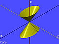
  Elliptic cone

• 

  Parabolic cylinder

• 

  Elliptic paraboloid

• 

  Hyperbolic paraboloid

• 

  Hyperboloid of one sheet

• 

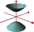
  Hyperboloid of two sheets

As trisectrix

A parabola can be used as a trisectrix, that is it allows the exact trisection of an arbitrary angle with straightedge and compass. This is not in contradiction to the impossibility of an angle trisection with compass-and-straightedge constructions alone, as the use of parabolas is not allowed in the classic rules for compass-and-straightedge constructions.

To trisect ${\displaystyle \angle AOB}$, place its leg ${\displaystyle OB}$ on the x axis such that the vertex ${\displaystyle O}$ is in the coordinate system's origin. The coordinate system also contains the parabola ${\displaystyle y=2x^{2}}$. The unit circle with radius 1 around the origin intersects the angle's other leg ${\displaystyle OA}$, and from this point of intersection draw the perpendicular onto the y axis. The parallel to y axis through the midpoint of that perpendicular and the tangent on the unit circle in ${\displaystyle (0,1)}$ intersect in ${\displaystyle C}$. The circle around ${\displaystyle C}$ with radius ${\displaystyle OC}$ intersects the parabola at ${\displaystyle P_{1}}$. The perpendicular from ${\displaystyle P_{1}}$ onto the x axis intersects the unit circle at ${\displaystyle P_{2}}$, and ${\displaystyle \angle P_{2}OB}$ is exactly one third of ${\displaystyle \angle AOB}$.

The correctness of this construction can be seen by showing that the x coordinate of ${\displaystyle P_{1}}$ is ${\displaystyle \cos(\alpha )}$. Solving the equation system given by the circle around ${\displaystyle C}$ and the parabola leads to the cubic equation ${\displaystyle 4x^{3}-3x-\cos(3\alpha )=0}$. The triple-angle formula ${\displaystyle \cos(3\alpha )=4\cos(\alpha )^{3}-3\cos(\alpha )}$ then shows that ${\displaystyle \cos(\alpha )}$ is indeed a solution of that cubic equation.

This trisection goes back to René Descartes, who described it in his book La Géométrie (1637).^[18]

Generalizations

If one replaces the real numbers by an arbitrary field, many geometric properties of the parabola ${\displaystyle y=x^{2}}$ are still valid:

1. A line intersects in at most two points.
2. At any point ${\displaystyle (x_{0},x_{0}^{2})}$ the line ${\displaystyle y=2x_{0}x-x_{0}^{2}}$ is the tangent.

Essentially new phenomena arise, if the field has characteristic 2 (that is, ${\displaystyle 1+1=0}$): the tangents are all parallel.

In algebraic geometry, the parabola is generalized by the rational normal curves, which have coordinates (x, x², x³, …, xⁿ); the standard parabola is the case n = 2, and the case n = 3 is known as the twisted cubic. A further generalization is given by the Veronese variety, when there is more than one input variable.

In the theory of quadratic forms, the parabola is the graph of the quadratic form x² (or other scalings), while the elliptic paraboloid is the graph of the positive-definite quadratic form x² + y² (or scalings), and the hyperbolic paraboloid is the graph of the indefinite quadratic form x² − y². Generalizations to more variables yield further such objects.

The curves y = x^p for other values of p are traditionally referred to as the higher parabolas and were originally treated implicitly, in the form x^p = ky^q for p and q both positive integers, in which form they are seen to be algebraic curves. These correspond to the explicit formula y = x^p/q for a positive fractional power of x. Negative fractional powers correspond to the implicit equation x^py^q = k and are traditionally referred to as higher hyperbolas. Analytically, x can also be raised to an irrational power (for positive values of x); the analytic properties are analogous to when x is raised to rational powers, but the resulting curve is no longer algebraic and cannot be analyzed by algebraic geometry.

In the physical world

In nature, approximations of parabolas and paraboloids are found in many diverse situations. The best-known instance of the parabola in the history of physics is the trajectory of a particle or body in motion under the influence of a uniform gravitational field without air resistance (for instance, a ball flying through the air, neglecting air friction).

The parabolic trajectory of projectiles was discovered experimentally in the early 17th century by Galileo, who performed experiments with balls rolling on inclined planes. He also later proved this mathematically in his book Dialogue Concerning Two New Sciences.^[19][h] For objects extended in space, such as a diver jumping from a diving board, the object itself follows a complex motion as it rotates, but the center of mass of the object nevertheless moves along a parabola. As in all cases in the physical world, the trajectory is always an approximation of a parabola. The presence of air resistance, for example, always distorts the shape, although at low speeds, the shape is a good approximation of a parabola. At higher speeds, such as in ballistics, the shape is highly distorted and doesn't resemble a parabola.

Another hypothetical situation in which parabolas might arise, according to the theories of physics described in the 17th and 18th centuries by Sir Isaac Newton, is in two-body orbits, for example, the path of a small planetoid or other object under the influence of the gravitation of the Sun. Parabolic orbits do not occur in nature; simple orbits most commonly resemble hyperbolas or ellipses. The parabolic orbit is the degenerate intermediate case between those two types of ideal orbit. An object following a parabolic orbit would travel at the exact escape velocity of the object it orbits; objects in elliptical or hyperbolic orbits travel at less or greater than escape velocity, respectively. Long-period comets travel close to the Sun's escape velocity while they are moving through the inner Solar system, so their paths are nearly parabolic.

Approximations of parabolas are also found in the shape of the main cables on a simple suspension bridge. The curve of the chains of a suspension bridge is always an intermediate curve between a parabola and a catenary, but in practice the curve is generally nearer to a parabola due to the weight of the load (i.e. the road) being much larger than the cables themselves, and in calculations the second-degree polynomial formula of a parabola is used.^[20][21] Under the influence of a uniform load (such as a horizontal suspended deck), the otherwise catenary-shaped cable is deformed toward a parabola (see Catenary#Suspension bridge curve). Unlike an inelastic chain, a freely hanging spring of zero unstressed length takes the shape of a parabola. Suspension-bridge cables are, ideally, purely in tension, without having to carry other forces, for example, bending. Similarly, the structures of parabolic arches are purely in compression.

Paraboloids arise in several physical situations as well. The best-known instance is the parabolic reflector, which is a mirror or similar reflective device that concentrates light or other forms of electromagnetic radiation to a common focal point, or conversely, collimates light from a point source at the focus into a parallel beam. The principle of the parabolic reflector may have been discovered in the 3rd century BC by the geometer Archimedes, who, according to a dubious legend,^[22] constructed parabolic mirrors to defend Syracuse against the Roman fleet, by concentrating the sun's rays to set fire to the decks of the Roman ships. The principle was applied to telescopes in the 17th century. Today, paraboloid reflectors can be commonly observed throughout much of the world in microwave and satellite-dish receiving and transmitting antennas.

In parabolic microphones, a parabolic reflector is used to focus sound onto a microphone, giving it highly directional performance.

Paraboloids are also observed in the surface of a liquid confined to a container and rotated around the central axis. In this case, the centrifugal force causes the liquid to climb the walls of the container, forming a parabolic surface. This is the principle behind the liquid-mirror telescope.

Aircraft used to create a weightless state for purposes of experimentation, such as NASA's "Vomit Comet", follow a vertically parabolic trajectory for brief periods in order to trace the course of an object in free fall, which produces the same effect as zero gravity for most purposes.

Gallery

• 

  A bouncing ball captured with a stroboscopic flash at 25 images per second. The ball becomes significantly non-spherical after each bounce, especially after the first. That, along with spin and air resistance, causes the curve swept out to deviate slightly from the expected perfect parabola.

• 

  Parabolic trajectories of water in a fountain.

• 

  The path (in red) of Comet Kohoutek as it passed through the inner Solar system, showing its nearly parabolic shape. The blue orbit is the Earth's.

• 

  The supporting cables of suspension bridges follow a curve that is intermediate between a parabola and a catenary.

• 

  The Rainbow Bridge across the Niagara River, connecting Canada (left) to the United States (right). The parabolic arch is in compression and carries the weight of the road.

• 

  Parabolic arches used in architecture

• 

  Parabolic shape formed by a liquid surface under rotation. Two liquids of different densities completely fill a narrow space between two sheets of transparent plastic. The gap between the sheets is closed at the bottom, sides and top. The whole assembly is rotating around a vertical axis passing through the centre. (See Rotating furnace)

• 

  Solar cooker with parabolic reflector

• 

  Parabolic antenna

• 

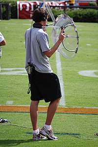
  Parabolic microphone with optically transparent plastic reflector used at an American college football game.

• 

  Array of parabolic troughs to collect solar energy

• 

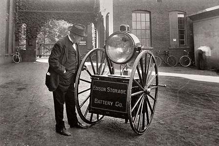
  Edison's searchlight, mounted on a cart. The light had a parabolic reflector.

• 

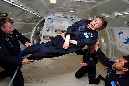
  Physicist Stephen Hawking in an aircraft flying a parabolic trajectory to simulate zero gravity

See also

• Degenerate conic
• Parabolic dome
• Parabolic partial differential equation
• Quadratic equation
• Quadratic function
• Universal parabolic constant

Footnotes

References

Further reading

• Lockwood, E. H. (1961). A Book of Curves. Cambridge University Press.

External links

• "Parabola", Encyclopedia of Mathematics, EMS Press, 2001 [1994]
• Weisstein, Eric W. "Parabola". MathWorld.
• Interactive parabola-drag focus, see axis of symmetry, directrix, standard and vertex forms
• Archimedes Triangle and Squaring of Parabola at cut-the-knot
• Two Tangents to Parabola at cut-the-knot
• Parabola As Envelope of Straight Lines at cut-the-knot
• Parabolic Mirror at cut-the-knot
• Three Parabola Tangents at cut-the-knot
• Focal Properties of Parabola at cut-the-knot
• Parabola As Envelope II at cut-the-knot
• The similarity of parabola at Dynamic Geometry Sketches, interactive dynamic geometry sketch.
• Frans van Schooten: Mathematische Oeffeningen, 1659

References

- ^ "Can You Really Derive Conic Formulae from a Cone? – Deriving the Symptom of the Parabola – Mathematical Association of America". Retrieved 30 September 2016.
- ^ Wilson, Ray N. (2004). Reflecting Telescope Optics: Basic design theory and its historical development (2 ed.). Springer. p. 3. ISBN 3-540-40106-7. Extract of page 3.
- ^ Stargazer, p. 115.
- ^ Stargazer, pp. 123, 132.
- ^ Fitzpatrick, Richard (July 14, 2007). "Spherical Mirrors". Electromagnetism and Optics, lectures. University of Texas at Austin. Paraxial Optics. Retrieved October 5, 2011.
- ^ a b Kumpel, P. G. (1975), "Do similar figures always have the same shape?", The Mathematics Teacher, 68 (8): 626–628, doi:10.5951/MT.68.8.0626, ISSN 0025-5769.
- ^ Shriki, Atara; David, Hamatal (2011), "Similarity of Parabolas – A Geometrical Perspective", Learning and Teaching Mathematics, 11: 29–34.
- ^ a b Tsukerman, Emmanuel (2013). "On Polygons Admitting a Simson Line as Discrete Analogs of Parabolas" (PDF). Forum Geometricorum. 13: 197–208.