오차함수

오차함수
오차 함수의 그림
일반정보
일반정의	${\displaystyle \operatorname {erf} z={\frac {2}{\sqrt {\pi}}\int_{0}^{z}e^{-t^{2}}\,\mathrm {d} t}$
응용분야	확률, 열역학
도메인, 코드 도메인 및 이미지
도메인	${\displaystyle \mathbb {R}}$
이미지	${\displaystyle \left (-1,1\right)}$
기본특징
패리티	이상한
특장점
뿌리	0
도함수	${\displaystyle {\frac {\mathrm {d}}{\mathrm {d} z}\operatorname {erf} z={\frac {2}{\sqrt {\pi}}e^{-z^{2}}$
유도체	${\displaystyle \int \operatorname {erf} z\, dz=z\operatorname {erf} z+{\frac {e^{-z^{2}}}{\sqrt {\pi}}+C}$
계열정의
테일러 급수	${\displaystyle \operatorname {erf} z={\frac {2}{\sqrt {\pi}}\sum _{n=0}^{\infty}{\frac {z}{2n+1}}\prod _{k=1}^{n}{\frac {-z^{2}}{k}}$

수학에서 오차 함수(, )는 다음과 같이 정의되는 복소 변수의 복소 함수입니다.^[1]

${\displaystyle \operatorname {erf} z={\frac {2}{\sqrt {\pi}}\int_{0}^{z}e^{-t^{2}}\,\mathrm {d} t.}$

일부 저자는 ${\displaystyle \mathrm{erf}}$ ${\displaystyle \operatorname {erf}}을($를) $2$ /${\displaystyle }$π ${\displaystyle$ 2$/{\sqrt {\pi}}$의 인수 없이 정의합니다$.$ 이 비요소적분은 확률, 통계 및 편미분 방정식에서 자주 발생하는 시그모이드 함수입니다.이러한 많은 응용 프로그램에서 함수 인수는 실수입니다.함수 인수가 real이면 함수 값도 real입니다.

통계량에서 x의 음이 아닌 값의 경우 오차 함수는 다음과 같이 해석됩니다. 평균이 0이고 표준 편차가 1/ √2인 정규 분포인 랜덤 변수 Y의 경우 erf x는 Y가 [-x, x] 범위에 속할 확률입니다.

밀접하게 관련된 두 가지 함수는 다음과 같이 정의된 상보적 오류 함수(erfc)입니다.

${\displaystyle \operatorname {erfc} z=1-\operatorname {erf} z,}$

그리고 가상 오차 함수(erfi)는 다음과 같이 정의됩니다.

${\displaystyle \operatorname {erfi} z=-i\operatorname {erf} iz,}$

여기서 i는 상상의 단위입니다.

이름.

오류함수라는 이름과 그 약칭 erf는 1871년 J. W. L. 글레이셔가 "확률론, 특히 오류론"과의 연관성 때문에 제안했습니다.^[3]오류 함수 보완은 Glaisher가 같은 해에 별도의 출판물을 통해서도 논의되었습니다.^[4]밀도가 다음과 같이 주어진 오차의 "설비 법칙"에 대하여

${\displaystyle f(x)=\left ({\frac {c}{\pi}}\right)^{\frac {1}{2}}^{-cx^{2}}}$

(정규 분포), Glaisher는 p와 q 사이에 오차가 있을 확률을 다음과 같이 계산합니다.

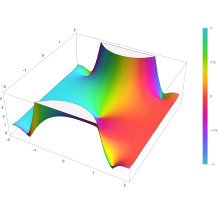
${\displaystyle \left ({\frac {c}{\pi}}\right)^{\frac {1}{2}}\int_{p}^{q}e^{-cx^{2}}\,\mathrm {d} x={\tfrac {1}{2}\left(\operatorname {erf} \left(q{\sqrt {c}\right)-\operatorname {erf} \left(p{\sqrt {c}\right)\right).$

적용들

일련의 측정 결과가 표준 편차 σ 및 기대 값이 0인 정규 분포로 설명될 때, erf(a/ σ √2)는 양의 a에 대해 단일 측정값의 오차가 -a와 +a 사이에 있을 확률입니다.이는 예를 들어, 디지털 통신 시스템의 비트 에러율(bit error rate)을 결정할 때 유용합니다.

오차 및 상보 오차 함수는 예를 들어 Heaviside step 함수에 의해 경계 조건이 주어질 때 열 방정식의 해에서 발생합니다.

오차 함수와 그 근사치는 높은 확률 또는 낮은 확률로 고정되는 결과를 추정하는 데 사용될 수 있습니다.임의 변수 X ~ Norm[μ, σ](평균 μ 및 표준 편차 σ를 갖는 정규 분포) 및 상수 L < μ:

${\displaystyle {\begin{aligned}\Pr[X\leq L]&={\frac {1}{2}}+{\frac {1}{2}}\operatorname {erf}{\f}{\frac {L-\mu }{\sqrt {2}\sigma }}\&\approx A\exp \left(-B\left({\frac {L-\mu }{\right)^{2}\right)\end{aligned}}$

여기서 A와 B는 특정 숫자 상수입니다.L이 평균, 구체적으로 μ - L ≥ σ√lnk에서 충분히 멀리 떨어져 있는 경우:

${\displaystyle \Pr[X\leq L]\leq A\exp(-B\ln {k})={\frac {A}{k^{B}}}}$

따라서 확률은 0으로 → ∞를 묻습니다.

X가 구간 [L_a, L_b]에 있을 확률은 다음과 같이 도출될 수 있습니다.

${\displaystyle {\begin{aligned}\Pr[L_{a}\leq X\leq L_{b}]&=\int _{L_{a}}^{L_{b}}{\frac {1}{\sqrt {2\pi}}\sigma }\exp \left (-{\frac {(x-\mu )^{2}}\right)\,\mathrm {d} x\&={\frac {1}{2}}\left(\operatorname {erf}{L_{b}-\mu }{{\sqrt {2}}}-\operatorname {erf}{\f}{\frac {L_{a}-\mu}{{\sqrt {2}}\right}\frac {L_{mu}{\sqrt {2}}\right.\end{aligned}}$

특성.

속성 erf(-z) = -erfz는 오차 함수가 홀수 함수임을 의미합니다.이는 적분이^−t2 짝수 함수라는 사실( 원점에서 0인 짝수 함수의 미분은 홀수 함수이며 그 반대)에서 직접적으로 비롯됩니다.

오차 함수는 실수를 실수로 바꾸는 전체 함수이므로, 임의의 복소수 z에 대하여:

${\displaystyle \operatorname {erf} {\overline {z}}={\overline {\operatorname {erf} z}}$

여기서 z는 z의 복소수 켤레입니다.

적분기 f = exp (-z)와 f = erfz는 도메인 컬러링으로 오른쪽 그림의 복소 z 평면에 표시됩니다.

+ ∞에서 오차 함수는 정확히 1입니다(가우스 적분 참조).실제 축에서 erf z는 z → +∞에서 단위에 접근하고 z → -∞에서 -1에 접근합니다.가상 축에서는 ±i ∞인 경향이 있습니다.

테일러 급수

오차 함수는 전체 함수이며, 특이점이 없고(무한대를 제외하고) 테일러 확장은 항상 수렴하지만, x > 1인 경우에는 잘못된 수렴으로 유명합니다.^[5]

정의적분은 기본함수의 관점에서 닫힌 형태로 평가될 수 없지만, 적분을^−z2 매클로린 급수로 확장하고 항마다 적분함으로써 오차함수의 매클로린 급수를 다음과 같이 구합니다.

${\displaystyle {\begin{aligned}\operatorname {erf} z&={\frac {2}{\sqrt {\pi}}\sum_{n=0}^{\infty}{\frac {(-1)^{n}z^{2n+1}}{n!(2n+1)}}\[6pt]&={\frac {2}{\sqrt {\pi }}\left(z-{\frac {z^{3}}}+{\frac {z^{5}{10}}-{\frac {z^{7}}}+{\frac {z^{9}{216}-\cdots \right)\end{align}}}$

모든 복소수 z를 의미합니다.분모항은 OEIS의 시퀀스 A007680입니다.

위의 영상 시리즈를 반복적으로 계산하려면 다음과 같은 대체 공식이 유용할 수 있습니다.

${\displaystyle {\begin{aligned}\operatorname {erf} z&={\frac {2}{\sqrt {\pi}}\sum_{n=0}^{\infty}\left(z\prod_{k=1}^{n}{\frac {-(2k-1)z^{2}}\right)\\[6pt]&={\frac {2}{\sqrt {\pi}}\sum _{n=0}^{\infty}{\frac {z}{2n+1}}\prod_{k=1}^{n}{\frac {-z^{2}}{k}}\end{aligned}}$

-(2k - 1)z/k(2k + 1)는 k번째 항을 (k + 1)번째 항(첫번째 항으로 consid링 z)으로 바꾸는 승수를 표현하기 때문입니다.

가상 오차 함수는 매클로린 급수와 매우 유사하며, 다음과 같습니다.

${\displaystyle {\begin{aligned}\operatorname {erfi} z&={\frac {2}{\sqrt {\pi}}\sum_{n=0}^{\infty}{\frac {z^{2n+1}}{n!(2n+1)}\[6pt]&={\frac {2}{\sqrt {\pi}}\left(z+{\frac {z^{3}}}+{\frac {z^{5}}{10}}+{\frac {z^{7}}{42}}+{\frac {z^{9}}+\cdots \right)\end{aligned}}$

모든 복소수 z를 의미합니다.

도함수와 적분

오류 함수의 도함수는 정의 직후에 나타납니다.

${\displaystyle {\frac {\mathrm {d}}{\mathrm {d} z}\operatorname {erf} z={\frac {2}{\sqrt {\pi}}e^{-z^{2}}}$

이로부터 가상 오차 함수의 도함수 또한 즉시 다음과 같습니다.

${\displaystyle {\frac {d}{dz}}\operatorname {erfi} z={\frac {2}{\sqrt {\pi}}}e^{z^{2}}}$

부품별로 적분하여 얻을 수 있는 오차 함수의 유도체는

${\displaystyle z\operatorname {erf} z+{\frac {e^{-z^{2}}{\sqrt {\pi}}}}$

허수 오차 함수의 유도체는 또한 부품들에 의해 적분됨으로써 얻을 수 있습니다.

${\displaystyle z\operatorname {erfi} z-{\frac {e^{z^{2}}{\sqrt {\pi}}}}$

고차 파생 상품은 다음과 같이 제공됩니다.

${\displaystyle \operatorname {erf} ^{(k)}z={\frac {2 (-1)^{k-1}}{\sqrt {\pi }}{\mathit {H}_{k-1}(z)e^{-z^{2}}={\frac {2}{\sqrt {\pi }}{\frac {\mathrm {d}^{k-1}}{\mathrm {d}z^{k-1}}\left(e^{-z^{2}\right),\qquad k=1,2,\dots }$

여기서 H는 물리학자들의 헤르마이트 다항식입니다.^[6]

뷔르만 급수

테일러 팽창보다 모든 x의 실수 값에 대해 더 빠르게 수렴하는 ^[7]팽창은 한스 하인리히 뷔르만의 정리를 사용하여 얻어집니다.^[8]

${\displaystyle {\begin{aligned}\operatorname {erf} x&={\frac {2}}\operatorname {sgn} x\cdot {\sqrt {1-e^{-x^{2}}}}\left(1-e^{\frac {1}{12}}\left(1-e^{-x^{2}\right)-{\frac {7}{480}\left(1-e^{-x^{2}\right)^{2}-{\frac {5}{896}}\left(1-e^{-x^{2}}\right)^{3}-{\frac {787}{276480}}\left(1-e^{-x^{2}}\right)^{4}-\cdots \right)\\[10pt]&={\frac {2}{\sqrt {\pi}}\operatorname {sgn} x\cdot {\sqrt {1-e^{-x^{2}}}\left ({\frac {\sqrt {\pi}}{2}}+\sum _{k=1}^{\infty}c_{k}e^{-kx^{2}\right}.\end{aligned}}$

여기서 sgn은 기호 함수입니다.처음 두 계수만 유지하고 c = 31/200 및 c = -341/8000을 선택하면 결과 근사치는 0.0036127보다 작은 x = ±1.3796에서 가장 큰 상대 오차를 나타냅니다.

${\displaystyle \operatorname {erf} x\approx {\frac {2}{\sqrt {\pi}}\operatorname {sgn} x\cdot {\sqrt {1-e^{-x^{2}}}\left ({\frac {\sqrt {\pi}}{2}}+{\frac {31}{200}e^{-x^{2}}-{\frac {341}{8000}e^{-2x^{2}}\right}.$

역함수

복소수 z가 주어졌을 때, erf w = z를 만족하는 유일한 복소수 w가 없으므로, 참된 역함수는 다중값이 될 것입니다.그러나 -1 < x < 1에 대하여 다음을 만족시키는 유일한 실수가⁻¹ 있습니다.

${\displaystyle \operatorname {erf} \left(\operatorname {erf}^{-1}x\right)=x.}$

역오류 함수는 대개 도메인(-1,1)으로 정의되며, 많은 컴퓨터 대수 시스템에서 이 도메인으로 제한됩니다.그러나 매클로린 계열을^[9] 사용하여 복소평면의 디스크 z < 1까지 확장할 수 있습니다.

${\displaystyle \operatorname {erf} ^{-1}z=\sum _{k=0}^{\infty}{\frac {c_{k}}{2k+1}}\left ({\frac {\sqrt {\pi}}{2}}z\right)^{2k+1}}$

여기서 c = 1 및

${\displaystyle {\begin{aligned}c_{k}&=\sum _{m=0}^{k-1}}{\frac {c_{m}c_{k-1-m}}{{(m+1)}}\&=\left\{1,1,{\frac {7}{6}},{\frac {127}{90},{\frac {4369}{2520}},{\frac {34807}{16200}},\ldots \right\}.\end{aligned}}$

따라서 열 확장(일반적인 요인은 분자 및 분모에서 취소됨):

${\displaystyle \operatorname {erf} ^{-1}z={\frac {\sqrt {\pi }{2}}\left(z+{\frac {\pi }{12}}z^{3}+{\frac {7\pi ^{2}}{480}}z^{5}+{\frac {127\pi ^{3}}+{40320}}z^{\frac {4369\pi ^{4}}+{ 5806080}+{\frac {34807\pi ^5}}\frac {182476800}z^{11}+\cdots \right}.$

(취소 후 분자/분수는 OEIS의 OEIS: A092676/OEIS: A092677이며, 취소하지 않으면 OEIS: A002067에서 분자항이 부여됩니다.)± ∞에서 오차 함수의 값은 ±1과 같습니다.

z < 1의 경우 erf(erf z) = z가 있습니다.

역상보 오차 함수는 다음과 같이 정의됩니다.

${\displaystyle \operatorname {erfc} ^{-1}(1-z)=\operatorname {erf} ^{-1}z.}$

실수 x에 대하여 erfi(erfix) = x를 만족하는 유일한 실수 erfix가 있습니다. 역수 허수 오차 함수는 erfix로 정의됩니다.

임의의 실수 x에 대하여 뉴턴의 방법을 사용하여 erfix를⁻¹ 계산할 수 있고, -1 ≤ x ≤ 1에 대하여 다음과 같은 매클로린 급수가 수렴합니다.

${\displaystyle \operatorname {erfi} ^{-1}z=\sum _{k=0}^{\infty}{\frac {(-1)^{k}c_{k}}{2k+1}}\left ({\frac {\sqrt {\pi}}{2}}z\right)^{2k+1}}$

여기서 c는_k 위와 같이 정의됩니다.

점근적 팽창

큰 실수 x에 대한 상보적 오차 함수의 유용한 점근적 확장(따라서 유용한 점근적 확장은

${\displaystyle {\begin{aligned}\operatorname {erfc} x&={\frac {e^{-x^{2}}}{x{\sqrt {\pi}}}\left(1+\sum _{n=1}^{\infty}(-1)^{n}{\frac {1\cdot 3\cdot 5\cdot 5\cdot (2n-1)}{\left(2x^{2}\right)^{n}}\right)\\[6pt]&={\frac {e^{-x^{2}}}{x{\sqrt {\pi}}}}\sum _{n=0}^{\infty}(-1)^{n}{\frac {(2n-1)!!!}{\left(2x^{2}\right)^{n}},\end{aligned}}$

여기서 (2n - 1)!!!는 (2n - 1)의 이중 요인이며, (2n - 1)까지의 모든 홀수의 곱입니다.이 급수는 모든 유한 x마다 발산하며, 점근적 팽창으로서 그것의 의미는 어떤 정수 N ≥ 1에 대하여

${\displaystyle \operatorname {erfc} x={\frac {e^{-x^{2}}}{x{\sqrt {\pi}}}}\sum _{n=0}^{N-1}^{n}{\frac {(2n-1)!!!}{\left(2x^{2}\right)^{n}}+R_{N}(x)}$

나머지는 여기에

${\displaystyle R_{N}(x):={\frac {(-1)^{N}}{\sqrt {\pi}}}2^{1-2N}{\frac {(2N)!}{N!}}\int_{x}^{\infty}t^{-2N}e^{-t^{2}}\,\mathrm {d}t,}$

쉽게 귀납법, 글로 따라가는

${\displaystyle e^{-t^{2}}=-(2t)^{-1}\left(e^{-t^{2}}\right)'}$

부품별로 통합할 수 있습니다.

란다우 표기법에서, 나머지 항의 점근적 거동은

${\displaystyle R_{N}(x)=O\left(x^{-(1+2N))}e^{-x^{2}}\right)}$

x → ∞로서이는 다음을 통해 확인할 수 있습니다.

x의 값이 충분히 클 경우 erfc x의 좋은 근사치를 얻기 위해 이 점근적 확장의 처음 몇 항만 필요합니다(x의 값이 너무 크지 않을 경우 0에서 위의 테일러 확장은 매우 빠른 수렴을 제공함).

지속적인 분율 확장

상보적 오차 함수의 지속적인 분수 확장은 다음과 같습니다.^[11]

${\displaystyle \operatorname {erfc} z={\frac {z}{\sqrt {\pi}}}{e^{-z^{2}}}{\ cfrac {a_{1}}{1+{\ cfrac {a_{2}}{{z^{2}}+{\ cfrac {a_{3}}{1+\ dotsb}}}},\qquad a_{m}={\frac {m}{2}}}}.$

오차함수와 가우시안 밀도함수의 적분

${\displaystyle \int _{-\infty }^{\infty }\operatorname {erf}\left(ax+b\right){\frac {1}{\sqrt {2\pi \sigma ^{2}}}\exp \left (-{\frac {(x-\mu )^{2}}{2\sigma ^{2}\right)\,\mathrm {d} x=\operatorname {erf}{\frac {a\mu +b}{\sqrt {1+2a^{2}\sigma ^{2}}},\qquad a,b,\mu,\in \mathbb {R}}\xp\right)\,\mathrm {d} x=\operatorname {erf}{\f}{\frac {a\mu +b}},\qquad a,b,\mu \in \mathbb {R}}}$

Ng와 Geller와 관련된 것으로, 변수의 변화와 함께 섹션 4.3의^[12] 공식 13.

요인 급수

역 요인 시리즈:

${\displaystyle {\begin{aligned}\operatorname {erfc} z&={\frac {e^{-z^{2}}}{{\sqrt {\pi}}\,z}\sum _{n=0}^{\infty}{\frac {(-1)^{n}Q_{n}}{{{(z^{2}+1)}^{\bar {n}}}\&={\frac {e^{-z^{2}}}{{\sqrt {\pi}}\,z}}\left(1-{\frac {1}{2}}}{\frac {1}{(z^{2}+1}}}{\frac {1}{4}}{\frac {1}{(z^{2}+1)}}-\cdots \right)\end{aligned}}}$

Re(z²) > 0에 대하여 수렴합니다. 여기서

${\displaystyle {\begin{aligned}Q_{n}&{\overset {\text{def}}{{}={}}}{\frac {1}}{\Gamma \left ({\frac {1}{2}}\right)}}\int_{0}^{\infty }\cdots(\tau -1)\cdots(\tau -n+1)\tau ^{-{\frac {1}{2}}e^{-\tau }\,d\tau \&=\sum _{k=0}^{n}\left ({\tfrac {1}{2}}\right)^{\bar {k}}s(n,k),\end{aligned}}}$

z는ⁿ 상승 요인을 나타내고 s(n,k)는 첫 번째 유형의 부호가 있는 스털링 수를 나타냅니다.^[13][14]이중 요인을 포함하는 무한합에 의한 표현도 존재합니다.

${\displaystyle \operatorname {erf} z={\frac {2}{\sqrt {\pi}}\sum _{n=0}^{\infty}{\frac {(-2)^{n}(2n-1)!!!} {(2n+1)!}}:z^{2n+1}}$

수치 근삿값

기본 함수를 사용한 근사치

• 아브라모위츠와 스테건은 다양한 정확도에 대한 몇 가지 근사치를 제공합니다(식 7.1.25–28).이를 통해 주어진 애플리케이션에 적합한 가장 빠른 근사치를 선택할 수 있습니다.정확도를 높이기 위해서는 다음과 같습니다.

  ${\displaystyle \operatorname {erf} x\approx 1-{\frac {1}{\left(1+a_{1}x+a_{2)}x^{2}+a_{3}x^{3}+a_{4}x^{4}\right)^{4}},\qquad x\geq 0}$

  (최대 오차: 5x10⁻⁴)

  여기서 a = 0.278393, a = 0.230389, a = 0.000972, a = 0.078108

  ${\displaystyle \operatorname {erf} x\approx 1-\left(a_{1}t+a_{2}t^{2}+a_{3}t^{3}\right)e^{-x^{2}},\quad t={\frac {1}{1+px}},\qquad x\geq 0}$

  (최대오차: 2.5x10⁻⁵)

  여기서 p = 0. 47047, a = 0.3480242, a = -0.0958798, a = 0. 747856

  $${\displaystyle \operatorname {erf} x\approx 1-{\frac {1}{\left(1+a_{1}x+a_{2)}x^{2}+\cdots +a_{6}x^{6}\right)^{16}},\qquad x\geq 0}$$

  
  (최대오차 : 3x10⁻⁷)

  여기서 a = 0.0705230784, a = 0.0422820123, a = 0.0092705272, a = 0.0001520143, a = 0.0002765672, a = 0.0000430638

  $${\displaystyle \operatorname {erf} x\approx 1-\left(a_{1}t+a_{2}t^{2}+\cdots +a_{5}t^{5}\right)e^{-x^{2}},\quad t={\frac {1}{1+px}}}$$

  
  (최대오차 : 1.5x10⁻⁷)

  여기서 p = 0.3275911, a = 0.254829592, a = -0.284496736, a = 1.421413741, a = -1.453152027, a = 1.061405429

  이러한 근사치는 모두 x ≥ 0에 대해 유효합니다.음의 x에 대해 이러한 근사치를 사용하려면 erf x가 홀수 함수이므로 erf x = -erf (-x)를 사용합니다.
• 상보적 오차 함수에 대한 지수 경계와 순수 지수 근사치는 다음과^[15] 같이 주어집니다.

  ${\displaystyle {\begin{aligned}\operatorname {erfc} x&\leq {erfc} x&\leq {\tfrac {1}{2}}+{\tfrac {1}}^{-x^{2}},&\leq e^{-x^{2}},&\quad x&>0\\operatorname {erfc} x&\tfrac {1}^{6}}+{\tfrac {1}}^{-{\frac {4}}x^{2}},&\quad x&>0.\end{aligned}}$

• 위의 내용은 N항에서 정확도가 증가하는 N개 지수의 합으로 일반화되어 erfc x가 2Q ̃(erfc x)에 의해 정확하게 근사화되거나 경계화될 수 있습니다.

  ${\displaystyle {\tilde {Q}}(x)=\sum _{n=1}^{N}a_{n}e^{-b_{n}x^{2}}}$

  특히, 밀접하게 연관된 Q-함수에 대한 최소 최대 근사치 또는 경계를 산출하는 수치 계수 {(a,b)}를 해결하기 위한 체계적인 방법론이 있습니다: x ≥ 0에 대한 Q(x) ≈ Q ̃(x), Q(x) ≤ Q ̃ ̃(x).지수 근사치의 많은 변형에 대한 계수 {(a,b)}과 N = 25까지의 경계가 포괄적인 데이터 세트로 액세스를 열 수 있도록 공개되었습니다.
• x ∈ [0,∞]에 대한 상보적 오차 함수의 엄격한 근사치는 매개 변수 {A,B}의 적절한 선택에 대해 다음을 보여준 Karagiannidis & Lioumpas(2007)에 의해 제공됩니다.

  ${\displaystyle \operatorname {erfc} x\prox {\frac {\left(1-e^{-Ax}\right)e^{-x^{2}}{B{\sqrt {\pi}}}}{B{\sqrt {\pi}}}}$

  그들은 모든 x ≥ 0에 대해 좋은 근사치를 제공하는 {A,B} = {1.98,1.135}를 결정했습니다.특정 응용프로그램에 대한 정확도를 조정하거나 식을 엄격한 경계로 변환하기 위해 대체 계수를 사용할 수도 있습니다.^[19]
• 단항 하한은^[20]

  $${\displaystyle \operatorname {erfc} x\geq {\sqrt {\frac {2e}{\pi}}{\frac {\sqrt {\beta -1}}{\beta }}e^{-\beta x^{2}},\qquad x\geq 0,\quad \beta >1,}$$

  

  원하는 근사 간격에 대한 오차를 최소화하기 위해 파라미터 β를 선택할 수 있습니다.
• 세르게이 위니츠키는 그의 "글로벌 파데 근사"를 이용하여 또 다른 근사치를 제시했습니다.^{[21][22]: 2–3}

  ${\displaystyle \operatorname {erf} x\approx \operatorname {sgn} x\cdot {\sqrt {1-\exp \left (-x^{2}{\frac {4}{\pi }}+ax^{2}}{1+ax^{2}}}}\right)}}}$

  어디에

  ${\displaystyle a={\frac {8(\pi -3)}{3\pi(4-\pi )}}\approx 0.1400 12.}$

  이것은 0의 이웃과 무한의 이웃에서 매우 정확하도록 설계되었으며 상대오차는 모든 실수 x에 대하여 0.00035보다 작습니다. 대체값 a ≈ 0.147을 사용하면 최대 상대오차는 약 0.00013으로 줄어듭니다.

  이 근사치를 반전시켜 역오차 함수에 대한 근사치를 얻을 수 있습니다.

  ${\displaystyle \operatorname {erf} ^{-1}x\approx \operatorname {sgn} x\cdot {\sqrt {\left ({\frac {2}{\pi a}}+{\frac {\ln \left(1-x^{2}\right){2}}\right)^{2}-{\frac {\ln \left(1-x^{2}\right)}}{a}}}-\left ({\frac {2}{\pi a}}+{\frac {\ln \left(1-x^{2}\right)}{2}}\right)}}}.$

• 실제 인수에 대한 최대 오차가 1.2×10인⁻⁷ 근사치는 다음과 같습니다.^[24]

  ${\displaystyle \operatorname {erf} x={\begin{case}1-\tau &x\geq 0\\\tau -1&x<0\end{case}}}$

  와 함께

  ${\displaystyle {\begin{aligned}\tau &=t\cdot \exp \left (-x^{2}-1.26551223+1.00002368t+0.37409196t^{2}+0.09678418t^{3}-0.18628806t^{4}\right.\\&\left.\qquad \qquad \qquad +0.27886807t^{5}-1.13520398t^{6}+1.48851587t^{7}-0.82215223t^{8}+0.17087277t^{9}\right)\end{aligned}}$

  그리고.

  ${\displaystyle t={\frac {1}{1+{\frac {1}{2}} x }}}}$

• 절대값에서 최대 상대${\displaystyle {\mathrm{오차}}^{}}$가 2$$-$$$53$ {\$displaystyle 2$${\displaystyle ^\{-}$$53$${\displaystyle \}\}(}$≈${\displaystyle }$1.${\displaystyle 1^{}}$ ${\displaystyle {\times }^{}}$ ${\displaystyle {10}^{}}$-$$16) {\$displaystyle$ \$left(\대략$ $.1\times 10^{-16$}\right$)}$의 근사값은 $x$ ≥ ${\displaystyle 0}$ ${\displaystyle x\geq 0$

  ${\displaystyle {\begin{aligned}\operatorname {erfc} \left(x\right)&=\left ({\frac {0.56418958354775629}{x+2.06955023132914151}\right)\left ({\frac {x^{2}+2.71078540045147805x+5.80755613130301624}{x^{2}+3.47954057099518960x+12.06166887286239555}\right)\&\left ({\frac {x^{2}+3.4746951377439592x+12.074036406381411}{x^{2}+3.720683960225092x+8.44319781003968454}\right)\left ({\frac {x^{2}+4.00561509202259545x+9.3059665887898}{x^{2}+3.9022540294078x+6.3616309538464}\right)\&\left ({\frac {x^{2}+5.16722705817}\right).812584x+9.12661617673673262}{x^{2}+4.03296893109262491x+5.135785305681539}\right)\left ({\frac {x^{2}+5.95908795446633271x+9.19435612886969243}{x^{2}+4.112409429450885x+4.48640329408675}\right)e^{-x^{2}}\\end{aligned}}}$

  < 인경우 {\$displaystyle x<0$}

  ${\displaystyle \operatorname {erfc} \left(x\right)=2-\operatorname {erfc} \left (-x\right)}$

값표

x	erfx	1 - erfx
0	0	1
0.02	0.022564575	0.977435425
0.04	0.045111106	0.954888894
0.06	0.067621594	0.932378406
0.08	0.090078126	0.909921874
0.1	0.112462916	0.887537084
0.2	0.222702589	0.777297411
0.3	0.328626759	0.671373241
0.4	0.428392355	0.571607645
0.5	0.520499878	0.479500122
0.6	0.603856091	0.396143909
0.7	0.677801194	0.322198806
0.8	0.742100965	0.257899035
0.9	0.796908212	0.203091788
1	0.842700793	0.157299207
1.1	0.880205070	0.119794930
1.2	0.910313978	0.089686022
1.3	0.934007945	0.065992055
1.4	0.952285120	0.047714880
1.5	0.966105146	0.033894854
1.6	0.976348383	0.023651617
1.7	0.983790459	0.016209541
1.8	0.989090502	0.010909498
1.9	0.992790429	0.007209571
2	0.995322265	0.004677735
2.1	0.997020533	0.002979467
2.2	0.998137154	0.001862846
2.3	0.998856823	0.001143177
2.4	0.999311486	0.000688514
2.5	0.999593048	0.000406952
3	0.999977910	0.000022090
3.5	0.999999257	0.000000743

관련기능

상보오차함수

erfc로 표시된 상보적 오류 함수는 다음과 같이 정의됩니다.

${\displaystyle {\begin{aligned}\operatorname {erfc} x&=1-\operatorname {erf} x\[5pt]&={\frac {2}{\sqrt {\pi}}\int_{x}^{\infty}e^{-t^{2}\,\mathrm {d} t\[5pt]&=e^{-x^{2}\operatorname {erfcx} x,\end{aligned}}$

또한 erfcx를 정의합니다. 이 함수는^[26] erfc 대신 산술 언더플로우를^[26][27] 피하기 위해 사용할 수 있습니다.x ≥ 0에 대한 또 다른 형태의 erfc x는 발견자의 이름을 따서 크레이그 공식으로 알려져 있습니다.

${\displaystyle \operatorname {erfc}(x\mid x\geq 0)={\frac {2}{\pi}}\int_{0}^{\frac {\pi}{2}}\exp \left (-{\frac {x^{2}}{\sin ^{2}\theta}}\right),\mathrm {d} \theta}$

이 식은 x의 양의 값에 대해서만 유효하지만, 음의 값에 대해서는 erfc x = 2 - erfc (-x)와 함께 사용하여 erfc(x)를 구할 수 있습니다.이 형태는 적분 범위가 고정적이고 유한하다는 점에서 유리합니다.음이 아닌 두 변수의 합의 erfc에 대한 이 식을 확장하면 다음과 같습니다.^[29]

${\displaystyle \operatorname {erfc}(x+y\mid x,y\geq 0)={\frac {2}{\pi }}\int _{0}^{\frac {\pi }{2}}\exp \left (-{\frac {x^{2}}{\sin ^{2}\theta }}-{\frac {y^{2}}{\cos ^{2}\theta }}\right)\,\mathrm {d} \theta}$

허수오차함수

허수 에러 함수, 즉 derfi로 표시되며 다음과 같이 정의됩니다.

${\displaystyle {\begin{aligned}\operatorname {erfi} x&=-i\operatorname {erf} ix\[5pt]&={\frac {2}{\sqrt {\pi}}\int _{0}^{x}e^{t^{2}\,\mathrm {d}t\[5pt]&={\frac {2}{\sqrt {\pi}}e^{x^{2}D(x),\end{aligned}}$

여기서 D(x)는 도슨 함수(산술 오버플로를^[26] 피하기 위해 erfi 대신 사용할 수 있음)입니다.

"상상오류함수"라는 이름에도 불구하고 x가 실수일 때 erfix는 실수입니다.

임의의 복소 인수 z에 대해 오류 함수를 평가할 때, 결과적인 복소 오류 함수는 일반적으로 Faddeeva 함수로서 축척된 형태로 논의됩니다.

${\displaystyle w(z)=e^{-z^{2}}\operatorname {erfc}(-iz)=\operatorname {erfcx}(-iz).}$

누적분포함수

오류 함수는 축척 및 변환에 의해서만 다르기 때문에 일부 소프트웨어 언어에서는 norm(x)로 명명된 φ로 표시되는 표준 정규 누적 분포 함수와 본질적으로 동일합니다.실제로.

${\displaystyle {\begin{aligned}\Phi(x)&={\frac {1}{\sqrt {2\pi}}}\int_{-\infty}^{x}e^{\tfrac {-t^{2}}\,\mathrm {d}t\[6pt]&={\frac {1}{2}\left(1+\operatorname {erf}{\frac {x}{\sqrt {2}}\right)\n\nt_x}\nt_x}^{\infty}^{x}^{\tfrac {2}},\tfrac {d}\t\mathrm {d}t\[6pt]&={\frac {2}\right)\left(1+\operatorname {erf}{\f}{\frac {x}{\s\[6pt]&={\frac {1}{2}}\operator name {erfc}\left (-{\frac {x}{\sqrt {2}}\right)\end{aligned}}$

또는 erf와 erfc를 위해 재배열:

${\displaystyle {\begin{aligned}\operatorname {erf}(x)&=2\Phi \left(x{\sqrt {2}}\right)-1\[6pt]\operator name {erfc}(x)&=2\Phi \left(-x{\sqrt {2}}\right)\\&=2\left(1-\Phi \left(x{\sqrt {2}}\right)\right).\end{aligned}}$

따라서 오차 함수는 표준 정규 분포의 꼬리 확률인 Q-함수와도 밀접한 관련이 있습니다.Q-함수는 오차함수로 다음과 같이 표현할 수 있습니다.

${\displaystyle {\begin{aligned}Q(x)&={\frac {1}{2}}-{\frac {1}{2}}\operatorname {erf}{\frac {x}{\sqrt {2}}\&={\frac {1}{2}}\operatorname {erfc}{\frac {x}{\sqrt {2}}.\end{aligned}}$

φ의 역수는 정상 분위 함수 또는 프로빗 함수로 알려져 있으며 역오차 함수로 다음과 같이 표현될 수 있습니다.

${\displaystyle \operator name {probit}(p)=\Phi ^{-1}(p)={\sqrt {2}}\연산자 이름 {erf} ^{-1}(2p-1)=-{\sqrt {2}}\연산자 이름 {erfc} ^{-1}(2p)입니다.$

표준 정규 cdf는 확률과 통계학에서 더 자주 사용되고, 오차 함수는 수학의 다른 분야에서 더 자주 사용됩니다.

오차 함수는 Mittag-Leffler 함수의 특수한 경우이며, 또한 합류 초기하학 함수(Kummer's function)로 나타낼 수 있습니다.

${\displaystyle \operatorname {erf} x={\frac {2x}{\sqrt {\pi}}}M\left({\tfrac {1}{2}},{\tfrac {3}{2}},-x^{2}\right).}$

그것은 프레넬 적분의 관점에서 간단한 표현을 가지고 있습니다.^{[further explanation needed]}

정규화된 감마 함수 P와 불완전한 감마 함수에 관하여,

${\displaystyle \operatorname {erf} x=\operatorname {sgn} x\cdot P\left({\tfrac {1}{2}}, x^{2}\right)={\frac {\operatorname {sgn} x}{\sqrt {\pi}}\gamma \left ({\tfrac {1}{2}, x^{2}\right).}$

sgn x는 기호 함수입니다.

일반화오류함수

일부 저자들은 보다 일반적인 기능에 대해 논의합니다.^{[citation needed]}

${\displaystyle E_{n}(x)={\frac {n!}{\sqrt {\pi}}}\int_{0}^{x}e^{-t^{n}}\,\mathrm {d} t={\frac {n!}{\sqrt {\pi}}}\sum _{p=0}^{\infty}(-1)^{p}{\frac {x^{np+1}}{(np+1)p!}}.}$

주목할 만한 사례는 다음과 같습니다.

• E(x)는 원점을 지나는 직선입니다. E(x) = x/e
• E₂(x)는 오차 함수, erfx입니다.

n!으로 나눈 후 홀수 n에 대한 모든 E는_n 서로 유사하게 보입니다.마찬가지로, 짝수 n에 대한_n E는 n!으로 단순하게 나눈 후에 서로 유사하게 보입니다.n > 0에 대한 모든 일반화된 오차 함수는 그래프의 양 x 측에서 유사하게 보입니다.

이러한 일반화된 함수는 감마 함수와 불완전 감마 함수를 사용하여 x > 0에 대해 동등하게 표현할 수 있습니다.

${\displaystyle E_{n}(x)={\frac {1}{\sqrt {\pi}}}\Gamma(n)\left(\Gamma \left ({\frac {1}{n}}\right)-\Gamma \left ({\frac {1}{n}}, x^{n}\right)\right)\qquad x>0).$

따라서 오차 함수를 불완전 감마 함수의 관점에서 정의할 수 있습니다.

${\displaystyle \operatorname {erf} x=1-{\frac {1}{\sqrt {\pi}}\Gamma \left ({\tfrac {1}{2}}, x^{2}\right).}$

상보적 오류 함수의 적분을 반복했습니다.

보차 오차 함수의 반복 적분은 다음과^[30] 같이 정의됩니다.

${\displaystyle {\begin{aligned}\operatorname {i}^{n}\!\operatorname {erfc} z&=\int _{z}^{\infty}\operatorname {i}^{n-1}\!\operatorname {erfc} \zeta \,\mathrm {d} \zeta \[6pt]\operatorname {i}^{0}\!\operatorname {erfc} z&=\operatorname {erfc} z\\\operatorname {i}^{1}\!\operatorname {erfc} z&=\operatorname {ierfc} z={\frac {1}{\sqrt {\pi}}}e^{-z^{2}-z\operatorname {erfc} z\\\operatorname {i}^{2}\!\operatorname {erfc} z&={\tfrac {1}{4}}\left(\operatorname {erfc} z-2z\operatorname {ierfc} z\right)\\end{aligned}}$

일반적인 재발 공식은

${\displaystyle 2n\cdot \operatorname {i}^{n}\!\operatorname {erfc} z=\operatorname {i}^{n-2}\!\operatorname {erfc} z-2z\cdot \operatorname {i}^{n-1}\!\operatorname {erfc} z}$

그들은 파워 시리즈를 가지고 있습니다.

${\displaystyle \operatorname {i}^{n}\!\operatorname {erfc} z=\sum _{j=0}^{\infty}{\frac {(-z)^{j}}{2^{n-j}j!\,\Gamma \left(1+{\frac {n-j}{2}}\right)}},$

대칭적인 특성을 따르는 것.

${\displaystyle \operatorname {i}^{2m}\!\operatorname {erfc}(-z)=-\operatorname {i}^{2m}\!\operatorname {erfc} z+\sum _{q=0}^{m}{\frac {z^{2q}}{2^{2(m-q)-1}(2q)!(m-q)!}}$

그리고.

${\displaystyle \operatorname {i}^{2m+1}\!\operatorname {erfc}(-z)=\operatorname {i}^{2m+1}\!\operatorname {erfc} z+\sum _{q=0}^{m}{\frac {z^{2q+1}}{2^{2(m-q)-1}(2q+1)!(m-q)!}}.}$

구현

실제 논쟁의 실제 기능으로서.

• POSIX 호환 운영 체제에서 헤더math.h그리고 수학 도서관을 선언할 것입니다.libm기능을 제공할 것.erf그리고.erfc(이중 정밀도) 및 단일 정밀도 및 확장 정밀도 대응물erff,erfl그리고.erfcf,erfcl.^[31]

• GNU 과학 도서관은 다음을 제공합니다.erf,erfc,log(erf), 그리고 스케일 에러 함수.^[32]

복잡한 논변의 복잡한 함수로서

• libcerf, 복잡한 오류 함수를 위한 숫자 C 라이브러리, 복잡한 함수를 제공합니다.cerf,cerfc,cerfcx그리고 실제 기능들.erfi,erfcxMIT Faddeeva Package에 구현된 Faddeeva 함수를 기반으로 약 13-14자리 정밀도로.

참고 항목

관련기능

• 가우스 적분, 전체 실선에 걸쳐
• 가우스 함수, 도함수
• 도슨 함수, 재규격화된 허수 오차 함수
• 굿윈-스태튼 적분

확률상

• 정규분포
• 정규 누적 분포 함수, 크기가 조정되고 이동된 형태의 오차 함수
• Probit, 정규 CDF의 역함수 또는 분위함수
• Q-함수, 정규 분포의 꼬리 확률
• 표준점수

참고문헌

추가열람

• Abramowitz, Milton; Stegun, Irene Ann, eds. (1983) [June 1964]. "Chapter 7". Handbook of Mathematical Functions with Formulas, Graphs, and Mathematical Tables. Applied Mathematics Series. Vol. 55 (Ninth reprint with additional corrections of tenth original printing with corrections (December 1972); first ed.). Washington D.C.; New York: United States Department of Commerce, National Bureau of Standards; Dover Publications. p. 297. ISBN 978-0-486-61272-0. LCCN 64-60036. MR 0167642. LCCN 65-12253.
• Press, William H.; Teukolsky, Saul A.; Vetterling, William T.; Flannery, Brian P. (2007), "Section 6.2. Incomplete Gamma Function and Error Function", Numerical Recipes: The Art of Scientific Computing (3rd ed.), New York: Cambridge University Press, ISBN 978-0-521-88068-8
• Temme, Nico M. (2010), "Error Functions, Dawson's and Fresnel Integrals", in Olver, Frank W. J.; Lozier, Daniel M.; Boisvert, Ronald F.; Clark, Charles W. (eds.), NIST Handbook of Mathematical Functions, Cambridge University Press, ISBN 978-0-521-19225-5, MR 2723248.

외부 링크

• 오차함수 적분표